· 23 min read
Retrieval-Augmented Generation, from first principles
- RAG
- LLMs
- Vector search
- Information retrieval
Contents · 13 sections
- 01Why retrieve at all
- 02The shape of a RAG system
- 03Indexing: parsing and chunking
- 04Embeddings: meaning as geometry
- 05Searching fast: HNSW and friends
- 06Hybrid search: when words matter
- 07Reranking: precision after recall
- 08Augment, then generate
- 09Beyond the baseline
- 10Measuring it
- 11Where it breaks
- 12A minimal implementation
- 13References
A large language model knows what was in its training data, as of the day training stopped, compressed into its weights. It can’t see your company wiki, last week’s release notes or the contract signed this morning, and when you ask about them it will often answer anyway, fluently and wrongly. Retrieval-Augmented Generation (RAG) fixes this in an unglamorous way: before the model answers, look up the relevant text and put it in the prompt.
That one sentence hides a full search engine. This article goes through each part: how documents become searchable vectors, why similarity is a matter of angles, how a graph index finds neighbours among millions of points without checking them all, why keyword search still matters, what rerankers add, how to assemble a prompt that keeps the model honest, and how to measure whether any of it works. The figures are animated where the idea is a process. They loop, so you can watch them twice.
Why retrieve at all
There are two places a model can keep knowledge. Parametric memory is the weights: billions of numbers that encode facts statistically, with no index, no provenance and no way to edit a single fact cleanly. Non-parametric memory is an external store you can read, update and cite. The original RAG paper (Lewis et al., 2020) paired a seq2seq generator with a dense index of Wikipedia and showed that the combination beat a much larger model working from its weights alone on knowledge-heavy tasks. The general lesson has held up: don’t make the model remember what it can look up.
Concretely, retrieval buys you four things that fine-tuning does not:
- Freshness. Re-indexing a changed document takes seconds. Retraining takes days and a budget.
- Private data. The model never has to be trained on your documents. They stay in a store you control, behind your access rules.
- Attribution. Every claim can point to the passage it came from, so a reader can check it.
- Fewer hallucinations, not zero. A model given the right passage and told to stay inside it invents far less. A model given the wrong passage will confidently summarise the wrong passage. Retrieval quality becomes the ceiling on answer quality, which is why most of this article is about retrieval.
The shape of a RAG system
Every RAG system splits into two pipelines that share one data structure. Indexing runs offline, whenever the corpus changes: documents are parsed, cut into chunks, turned into vectors and written to an index. Querying runs online, once per question: the question is embedded with the same model, the index returns the nearest chunks, a reranker reorders them, and the best few are pasted into the prompt the LLM answers from.
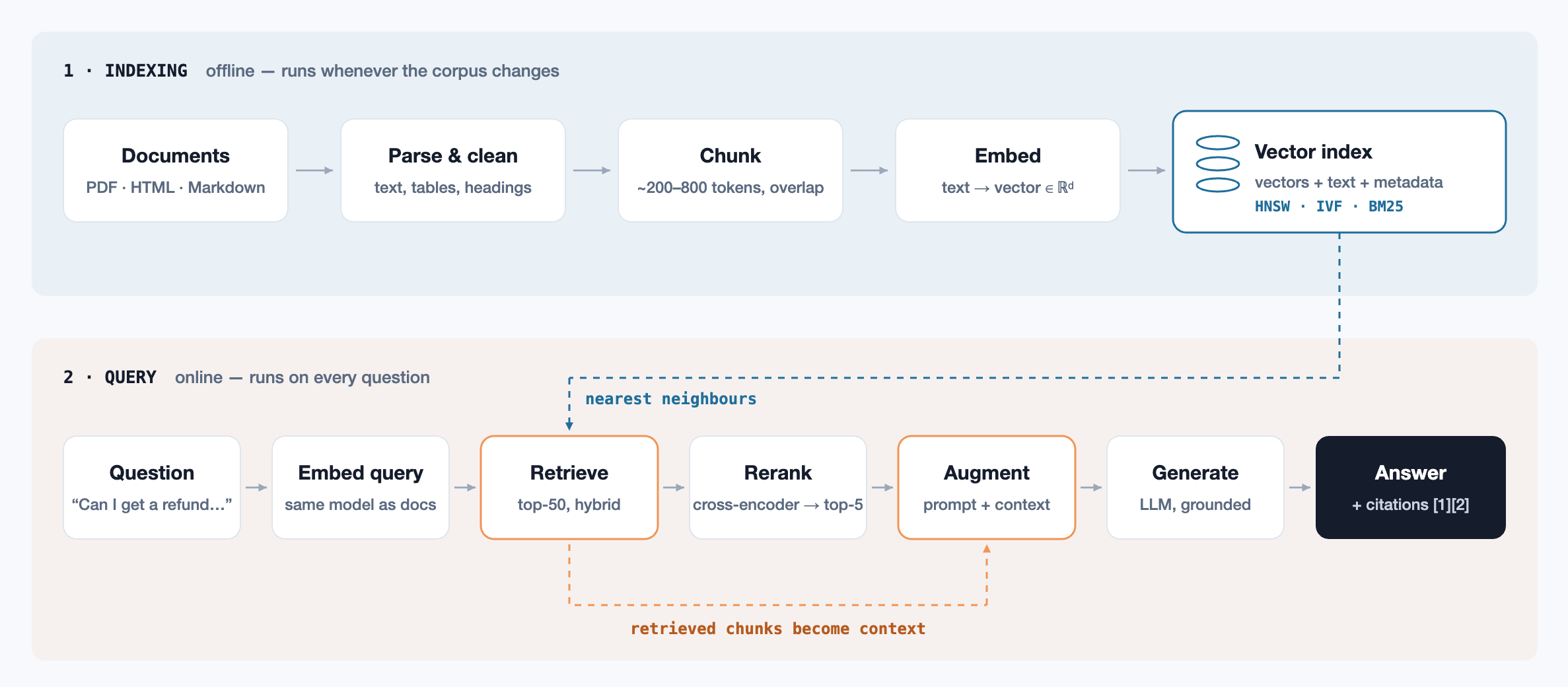
Here is the online half end to end, for one real-looking question. Watch the citations in the answer: each lights up the source card it came from. That link between claim and source is what you are building.
Indexing: parsing and chunking
Before anything is embedded it has to be text, and getting clean text out of real documents is where many systems quietly lose. PDFs put headers, footers and page numbers in the middle of sentences. Tables come out as a soup of cells. Two-column layouts get read straight across. Boilerplate (navigation, cookie banners, legal footers) repeats on every page and pollutes every search. A good parser keeps structure (headings, lists, table rows) and drops the rest. Time spent here pays off more than time spent tuning the embedding model.
Then the text is cut into chunks, the unit you retrieve. There are two reasons not to embed whole documents. Embedding models have input limits, and a single vector for a 40-page document is an average of everything in it, so it matches nothing well. Chunks that are too small have the opposite problem: “It is non-refundable.” is useless once you can’t see what “it” is.
Chunking strategies
- Fixed-size with overlap (Fig. 3). Simple and predictable, but blind to meaning: a boundary can land mid-sentence or split a table. The overlap, typically 10–20% of the size, is a cheap guard against that.
- Recursive splitting. Try to split on the largest natural separator (sections, then paragraphs, then sentences, then words), and only go to a finer one when a piece is still too big. This is the sensible default for prose.
- Structure-aware. Split on the document’s own structure: Markdown headings, HTML sections, function boundaries in code, rows in a table. Then carry the heading path along with each chunk (“Billing › Refunds › Annual plans”). This is usually the biggest single improvement on technical documentation.
- Semantic. Embed each sentence and start a new chunk where the similarity between neighbouring sentences drops, which is where the topic changes. More expensive, and helpful on long unstructured text such as transcripts.
Chunk size is a precision–context trade-off
Small chunks (100–250 tokens) give sharp embeddings and precise matches, but each one carries little context. Large chunks (500–1,000) carry context, but their embeddings blur over several ideas and they use up the prompt budget faster. Two patterns let you have both:
- Small-to-big (parent-document) retrieval: search over small chunks, but hand the LLM the larger section each one came from.
- Contextual chunk headers: before embedding, prepend a line that places the chunk in its document: title, section path, date. Anthropic’s “contextual retrieval” goes further and has an LLM write a one-sentence summary of each chunk’s place in the document. They report this roughly halved retrieval failures in their tests.
Whatever you choose, store metadata with each chunk: source, URL, section, last-modified date, language, access-control tags. Metadata filters (“only documents this user may see”, “only the v3 docs”) are applied at search time and are often worth more than any model upgrade.
Embeddings: meaning as geometry
An embedding model maps a piece of text to a vector of a few hundred to a few thousand numbers. It is trained (usually contrastively, on pairs of related texts such as a question and the passage that answers it) so that texts with similar meaning land close together and unrelated texts land far apart. After training, the geometry is the semantics. “How do I get my money back?” and “Refunds are issued to the original payment method” share no important words but sit close together in the space.
“Close” is usually measured with cosine similarity, the cosine of the angle between two vectors:
Normalise every vector to length 1 at index time and cosine similarity becomes a plain dot product, the cheapest operation there is. It also gives a useful picture: every embedding is a point on the surface of a high-dimensional sphere, and similarity is just how small the angle between two points is. Fig. 4 is that picture in two dimensions.
Choosing and using an embedding model
- Benchmarks are a shortlist, not an answer. The MTEB leaderboard ranks models across many retrieval tasks, but your corpus is not on it. Pick three candidates and test them on your own questions (see Measuring it).
- Queries and documents are asymmetric. A question is short and asks. A passage is long and states. Many models are trained for this and expect a prefix such as
query:/passage:, or have separate query and document modes. Leaving them out quietly costs accuracy. - Dimensions cost memory. 1M chunks × 1,024 float32 dimensions is 4 GB before index overhead. Matryoshka-trained models let you truncate vectors (say from 1,024 to 256) with modest loss, and quantising to int8 or binary cuts storage by 4–32×. Rescore the top candidates at full precision.
- Changing the model means re-embedding everything. Vectors from different models live in unrelated spaces. Version your index with the model name.
Searching fast: HNSW and friends
Exact nearest-neighbour search compares the query against every vector: O(N · d) per query. For 100k chunks that takes a few milliseconds and you should just do it. For 100M it doesn’t work. Approximate nearest neighbour (ANN) indexes give up a little recall (they may occasionally miss a true neighbour) to cut search cost from linear to roughly logarithmic.
The most widely used is HNSW, Hierarchical Navigable Small World graphs (Malkov & Yashunin, 2016). Every vector is a node in a proximity graph, linked to a handful of its near neighbours. Greedy search on such a graph works: from any node, keep moving to whichever neighbour is closer to the query until none is. But on a flat graph that walk takes many small steps. HNSW adds a hierarchy, much like a skip list. Each node is also placed on higher layers with exponentially decreasing probability, so the top layer has a few nodes connected by long links and the bottom layer has every node connected by short ones. Search starts at the top, makes long jumps to get near the query, then drops a layer and refines.
Fig. 5 shows the greedy core. Real HNSW keeps a candidate list of size efSearch instead of a single current node, because pure greedy descent can stop in a local minimum. For some random seeds of the graph in Fig. 5 it does exactly that. The parameters you will actually tune:
M: links per node. Higher gives better recall and more memory. 16–32 is typical.efConstruction: candidate list size while building. Higher makes a better graph and a slower build.efSearch: candidate list size at query time. This is the recall–latency dial you can turn per query without rebuilding.
The other main family is IVF (inverted file): k-means the vectors into a few thousand clusters, then at query time search only the nprobe clusters whose centroids are nearest. Combined with product quantisation (PQ), which splits each vector into sub-vectors and stores each as a one-byte code, IVF-PQ fits billions of vectors in memory at some cost in accuracy. HNSW is the default up to tens of millions of vectors in RAM. IVF-PQ and disk-based graph indexes take over beyond that.
Hybrid search: when words matter
Dense retrieval is good at paraphrase and bad at exactness. Ask about “error E1043” and an embedding model sees “some error code”. It may well rank a general troubleshooting page above the one page that names E1043. Product names, IDs, error codes, legal clause numbers and rare jargon are all cases where lexical search wins, and the standard lexical scorer is BM25:
Here f(t, D) is how often term t appears in document D, and IDF rewards rare terms. k1 (about 1.2–2) makes repeated occurrences count for less and less, and b (about 0.75) normalises for document length. A term like “E1043” that appears in one document out of a million gets a huge IDF, which is exactly the behaviour you want.
Hybrid search runs both retrievers and merges their results. The merge is the tricky part: BM25 scores are unbounded and cosine scores sit in a narrow band, so adding them is meaningless. Reciprocal Rank Fusion (Cormack et al., 2009) avoids the problem by ignoring scores and using only ranks:
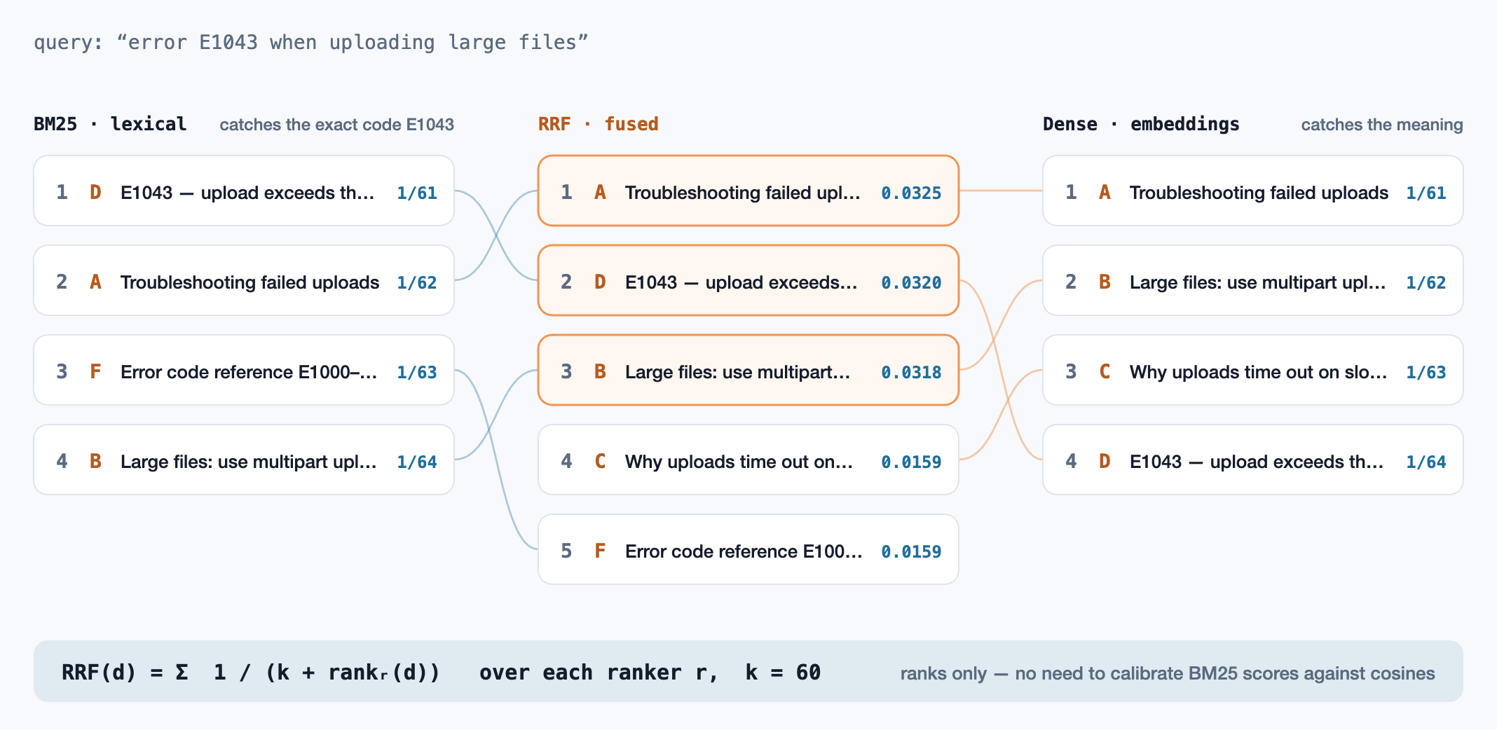
With k = 60, a document ranked first by one retriever scores 1/61. A document ranked well by both beats a document ranked first by only one, which is the agreement you are looking for. RRF needs no tuning, which is why it is the default in most search engines that support hybrid queries.
Reranking: precision after recall
The embedding model behind retrieval is a bi-encoder: query and document are encoded separately and compared with a dot product. That is what makes it fast, because document vectors are computed once, offline. It is also what limits it. The model never sees the query and the document together, so it can’t notice that the passage mentions refunds but only to say they don’t apply in this case.
A cross-encoder reads the pair together, [CLS] query [SEP] document, in one transformer pass, so every query token can attend to every document token. It outputs a single relevance score and is much more accurate (Nogueira & Cho, 2019). It is also far too slow to run over a corpus: one forward pass per document, per query, with nothing precomputable. So you use both in a funnel:
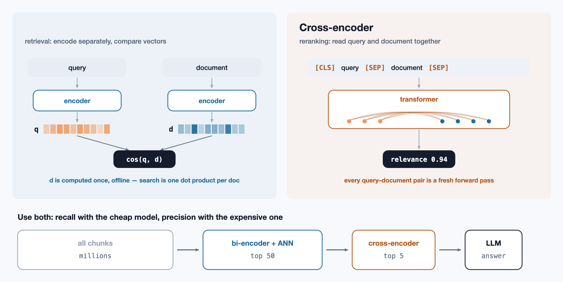
A typical setting retrieves 50–100 candidates with hybrid search and reranks them down to 3–8 for the prompt. Reranking is usually the single biggest quality improvement you can add to a working baseline. It also lets you be generous with first-stage recall, because junk in the top 50 is cheap now that something downstream filters it. (ColBERT-style late interaction models sit between the two: they store a vector per token and compare at token level, close to cross-encoder quality at a fraction of the cost.)
Augment, then generate
The “augmented” in RAG is prompt construction, and it deserves more care than it usually gets. A solid template has four parts:
- Instructions that set the rules: answer only from the context; cite sources as [n]; if the context doesn’t contain the answer, say so. That last instruction is what turns “confidently wrong” into “honestly unsure”.
- The context, delimited and numbered: wrap it in clear tags, give each chunk an id and its source, and keep the heading path so the model knows what “it” refers to.
- The question, plus any conversation history the question depends on. Rewrite follow-ups like “and for annual plans?” into standalone questions before retrieval, not after.
- An output contract: format, length, how to cite, how to handle sources that conflict (prefer the newest, or say they disagree).
Order matters. Liu et al. (2023) found that models use information at the start and end of a long context much better than information buried in the middle (“lost in the middle”). Put the best chunks first. Don’t pad the prompt to fill the window, either. Ten mediocre chunks often produce a worse answer than three good ones, because every irrelevant passage is a distraction the model has to ignore.
Citations are a product feature and a debugging tool. Users can check answers, and you can tell which chunk caused a bad one. Validate them after generation: every [n] must refer to a real chunk, and a cheap check that the cited chunk actually supports the sentence catches a surprising number of fabrications.
Beyond the baseline
Once the basic pipeline works and you can measure it, these are the upgrades worth knowing about:
- Query rewriting. Users write vague, conversational or misspelled queries. An LLM call that rewrites the query, or produces several variants and fuses their results with RRF (multi-query), lifts recall cheaply.
- HyDE (Gao et al., 2022). Have the LLM write a hypothetical answer, then embed that instead of the question. An answer-shaped text lands nearer to answer-shaped passages than a short question does. It works well when queries are short and documents are dense.
- Agentic / iterative retrieval. (How agents run this kind of loop is covered in the article on coding agents.) Some questions need several hops: “which of our customers on the legacy plan were affected by last month’s outage?” Let the model retrieve, read, decide what is missing and retrieve again, with a cap on steps. Self-RAG and similar methods train the model to decide when retrieval is needed at all.
- Structured and graph retrieval. Some questions are queries, not searches: “how many tickets mentioned E1043 last week?” Route those to SQL or an API. GraphRAG-style approaches build an entity graph and community summaries for questions about the corpus as a whole (“what are the main themes in these 2,000 interviews?”), which top-k chunk retrieval answers badly.
- Long context isn’t a replacement. Million-token windows make “just paste everything” work for small corpora, and you should use that when it fits. But retrieval still wins on cost, latency, freshness, access control and citability once the corpus outgrows the window, which most real ones do.
Measuring it
A RAG system can fail in two places, so evaluate them separately. Otherwise you can’t tell a retrieval bug from a generation bug.
Retrieval
Build a labelled set: 50–200 realistic questions, each with the chunk(s) that contain the answer. Write some by hand from real user logs, and generate more by asking an LLM to write questions about sampled chunks (then review them). Then measure:
- Recall@k: the fraction of questions where a relevant chunk appears in the top k. This is the metric that matters most, because if the answer isn’t retrieved nothing downstream can fix it.
- MRR (mean reciprocal rank): rewards putting the right chunk near the top.
nDCG is the standard when you have graded relevance (some chunks partly answer the question, some fully). Track these per change, across chunking, embedding model, hybrid weights and reranker, and keep only the changes that move them.
Generation
For answers, use an LLM as a judge with a narrow rubric. The RAGAS framework (Es et al., 2023) gives the common vocabulary:
- Faithfulness: is every claim in the answer supported by the retrieved context? This measures hallucination.
- Answer relevance: does the answer address the question that was asked?
- Context precision / recall: was the retrieved context relevant, and did it contain what a reference answer needed?
Calibrate the judge against a few dozen human labels before trusting it. Include questions whose answer is deliberately not in the corpus as well: a good system says “I don’t know” to those, and that is a behaviour you have to test for.
Where it breaks
When an answer is wrong, find the first stage that went wrong. Look at the retrieved chunks first: most failures are visible there.
| Symptom | Likely cause | First thing to try |
|---|---|---|
| Right document, wrong passage | Chunks too large, or split mid-thought | Structure-aware chunking; smaller chunks with parent-document expansion |
| Misses exact names, codes, IDs | Dense-only retrieval | Add BM25 and fuse with RRF |
| Relevant chunk at rank 30 | Bi-encoder imprecision | Retrieve more, add a cross-encoder reranker |
| Answer from an outdated doc | Stale index, no recency signal | Incremental re-indexing; date metadata; prefer-newest instruction |
| Fluent answer, unsupported claims | Weak grounding instructions, noisy context | Fewer, better chunks; “say you don’t know”; citation validation |
| Fine on single facts, fails on comparisons | Multi-hop question, single retrieval | Query decomposition or iterative retrieval |
| Chunk says “it” / “this plan” | Chunk lost its context | Contextual chunk headers |
| Leaks a document the user can’t see | Access control applied after retrieval, or not at all | Filter by permissions inside the search, every time |
A minimal implementation
Everything above, reduced to the parts that matter. It deliberately uses no framework: two function types stand in for whatever embedding model and LLM you use. Exact search with a dot product is honestly fine up to about a hundred thousand chunks. Swap in a vector database when you outgrow it, not before.
// Provider-agnostic: plug in any embedding model and any chat model.
export type Embed = (texts: string[]) => Promise<number[][]>;
export type Complete = (system: string, user: string) => Promise<string>;

export type Chunk = { id: string; source: string; text: string; vector: number[] };

// 1. Chunk: a fixed window of words with overlap. Use a structure-aware splitter for real docs.
export function chunk(source: string, text: string, size = 300, overlap = 60) {
  const words = text.split(/\s+/);
  const out: { id: string; source: string; text: string }[] = [];
  for (let start = 0; start < words.length; start += size - overlap) {
    out.push({ id: source + "#" + out.length, source, text: words.slice(start, start + size).join(" ") });
    if (start + size >= words.length) break;
  }
  return out;
}

// 2. Index: embed every chunk once, normalised so a dot product is a cosine.
export async function buildIndex(docs: { source: string; text: string }[], embed: Embed) {
  const pieces = docs.flatMap((d) => chunk(d.source, d.text));
  const vectors = await embed(pieces.map((p) => p.text));
  return pieces.map((p, i) => ({ ...p, vector: normalise(vectors[i]) }));
}

const normalise = (v: number[]) => {
  const n = Math.hypot(...v);
  return v.map((x) => x / n);
};
const dot = (a: number[], b: number[]) => a.reduce((s, x, i) => s + x * b[i], 0);

// 3. Retrieve: exact search. Fine to ~100k chunks; past that, hand this to an ANN index.
export async function retrieve(index: Chunk[], query: string, embed: Embed, k = 5) {
  const [q] = await embed([query]);
  const qn = normalise(q);
  return index
    .map((c) => ({ chunk: c, score: dot(qn, c.vector) }))
    .sort((a, b) => b.score - a.score)
    .slice(0, k);
}

// 4. Fuse two rankings (say BM25 and dense) by reciprocal rank.
export function rrf(rankings: string[][], k = 60) {
  const score = new Map<string, number>();
  for (const ranking of rankings)
    ranking.forEach((id, r) => score.set(id, (score.get(id) ?? 0) + 1 / (k + r + 1)));
  return [...score.entries()].sort((a, b) => b[1] - a[1]).map(([id]) => id);
}

// 5. Augment and generate: number the sources so the answer can cite them.
export async function answer(index: Chunk[], question: string, embed: Embed, complete: Complete) {
  const hits = await retrieve(index, question, embed);
  const context = hits
    .map((h, i) => "[" + (i + 1) + "] (" + h.chunk.source + ")\n" + h.chunk.text)
    .join("\n\n");
  const system =
    "Answer using only the context below. Cite every claim as [n]. " +
    "If the context does not contain the answer, say you don't know.\n\n<context>\n" +
    context + "\n</context>";
  return { text: await complete(system, question), sources: hits.map((h) => h.chunk.source) };
}
And the retrieval half of evaluation, which you should write before you tune anything:
import { retrieve, type Chunk, type Embed } from "./rag";

// Retrieval quality on a labelled set: for each question, which chunk ids hold the answer.
type Case = { question: string; relevant: Set<string> };

export async function evaluate(index: Chunk[], cases: Case[], embed: Embed, k = 5) {
  let hits = 0, rr = 0;
  for (const c of cases) {
    const ids = (await retrieve(index, c.question, embed, k)).map((h) => h.chunk.id);
    const first = ids.findIndex((id) => c.relevant.has(id));
    if (first >= 0) { hits++; rr += 1 / (first + 1); }
  }
  return { recallAtK: hits / cases.length, mrr: rr / cases.length };
}
From here, improvement is an empirical loop: change one thing (chunking, the embedding model, adding BM25, adding a reranker), rerun the evaluation, and keep the change only if recall@k or faithfulness moves. RAG rewards that discipline more than cleverness. Most of the gains are in the parts of the pipeline nobody demos: clean parsing, sensible chunks, and a test set that reflects what users actually ask.
References
- Lewis, P. et al. (2020). Retrieval-Augmented Generation for Knowledge-Intensive NLP Tasks. NeurIPS. arXiv:2005.11401
- Karpukhin, V. et al. (2020). Dense Passage Retrieval for Open-Domain Question Answering. EMNLP. arXiv:2004.04906
- Malkov, Y. & Yashunin, D. (2016). Efficient and Robust Approximate Nearest Neighbor Search Using Hierarchical Navigable Small World Graphs. arXiv:1603.09320
- Jégou, H., Douze, M. & Schmid, C. (2011). Product Quantization for Nearest Neighbor Search. IEEE TPAMI. doi:10.1109/TPAMI.2010.57
- Robertson, S. & Zaragoza, H. (2009). The Probabilistic Relevance Framework: BM25 and Beyond. Foundations and Trends in Information Retrieval. doi:10.1561/1500000019
- Cormack, G., Clarke, C. & Büttcher, S. (2009). Reciprocal Rank Fusion Outperforms Condorcet and Individual Rank Learning Methods. SIGIR. doi:10.1145/1571941.1572114
- Nogueira, R. & Cho, K. (2019). Passage Re-ranking with BERT. arXiv:1901.04085
- Khattab, O. & Zaharia, M. (2020). ColBERT: Efficient and Effective Passage Search via Contextualized Late Interaction over BERT. SIGIR. arXiv:2004.12832
- Liu, N. F. et al. (2023). Lost in the Middle: How Language Models Use Long Contexts. arXiv:2307.03172
- Gao, L. et al. (2022). Precise Zero-Shot Dense Retrieval without Relevance Labels (HyDE). arXiv:2212.10496
- Kusupati, A. et al. (2022). Matryoshka Representation Learning. NeurIPS. arXiv:2205.13147
- Muennighoff, N. et al. (2022). MTEB: Massive Text Embedding Benchmark. arXiv:2210.07316
- Asai, A. et al. (2023). Self-RAG: Learning to Retrieve, Generate, and Critique through Self-Reflection. arXiv:2310.11511
- Edge, D. et al. (2024). From Local to Global: A Graph RAG Approach to Query-Focused Summarization. arXiv:2404.16130
- Es, S. et al. (2023). RAGAS: Automated Evaluation of Retrieval Augmented Generation. arXiv:2309.15217
- Anthropic (2024). Introducing Contextual Retrieval. anthropic.com/news/contextual-retrieval
Related reading
AI · 10 min read
Mixture-of-Experts: sparse models, routing and the cost of balance
How MoE layers route each token to a few experts: top-k gating, why routers collapse and how load-balancing losses and bias terms prevent it, expert capacity and dropped tokens, all-to-all communication, and total versus active parameters.
AI · 24 min read
Inside an AI coding agent: loops, attention, context and orchestration
How a coding agent keeps working on a task: the agent loop, why attention dilutes as context grows, context engineering and compaction, the KV cache, keeping long runs on track, and orchestrating roles as a DAG.
AI · 9 min read
From RLHF to DPO: the maths of preference training
Bradley–Terry reward models, PPO with a KL penalty, the closed-form optimum that lets DPO drop the reward model, reward hacking, and GRPO with verifiable rewards for reasoning models.