FlashAttention: making attention IO-aware

For years, long-context attention was “too expensive” because it is quadratic in sequence length. That was true, but it hid the real bottleneck. On a modern GPU, standard attention spends most of its time moving numbers between memory and compute, not multiplying them. FlashAttention (Dao et al., 2022) computes exactly the same result with a fraction of the memory traffic, and in doing so made today’s long context windows practical.

This article works through the idea from the hardware up: why attention is memory-bound, the memory hierarchy that makes tiling pay, the online-softmax trick that makes tiling possible for a row-wise normalisation, the IO analysis, the backward pass, and what FlashAttention-2 and -3 changed on newer GPUs.

Attention is memory-bound

For one head with sequence length N and head dimension d, attention is three steps:

The obvious implementation runs each step as a separate GPU kernel, writing S and P out to GPU memory and reading them back in. With N = 8,192, one head’s S is 67 million entries, 134 MB in FP16, written and read several times, for every head in every layer.

Whether an operation is limited by compute or by memory depends on its arithmetic intensity: FLOPs per byte moved. An A100 does about 312 TFLOP/s of FP16 matrix maths but moves only about 1.5–2 TB/s from its main memory, so anything that does fewer than roughly 150–200 FLOPs per byte waits on memory. The matrix multiplies in attention are fine. The softmax, the masking and the dropout are elementwise, a few FLOPs per element loaded, and they dominate the run time. Profiling standard attention shows the GPU’s arithmetic units mostly idle.

The GPU memory hierarchy

GPUs have two kinds of memory that matter here. HBM (high-bandwidth memory) is the “GPU memory” you see in the spec sheet: tens of gigabytes. SRAM is on the chip itself: a couple of hundred kilobytes per streaming multiprocessor (SM), about 20 MB across an A100, and an order of magnitude faster.

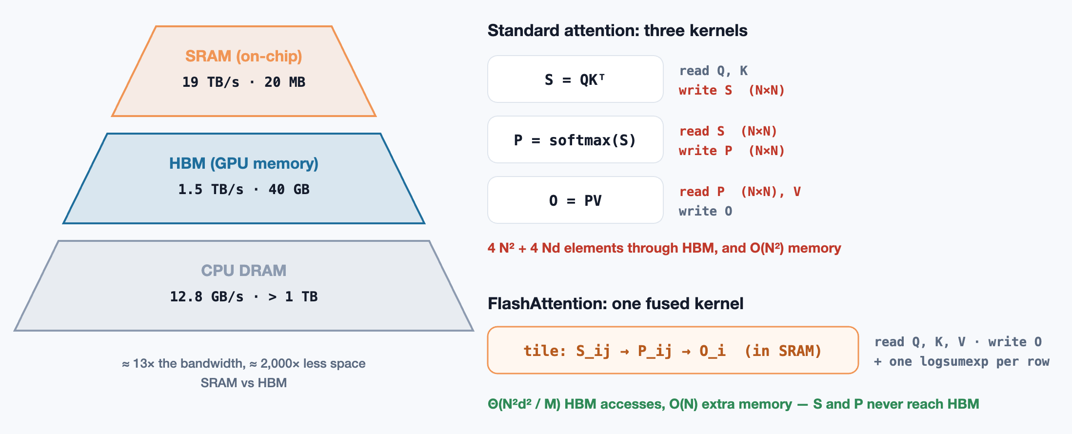
The whole game is to do as much work as possible per byte brought into SRAM. Kernel fusion (doing all three steps in one kernel) is the standard answer for elementwise chains. Attention resists it, because the softmax needs a whole row of S before it can normalise, and a row of length 8,192, times the 128 rows a thread block handles, does not fit in SRAM.

Tiling: never materialise S

FlashAttention splits Q into blocks of rows, and K and V into blocks of columns, each small enough to fit in SRAM. For a query block Q_i and a key/value block (K_j, V_j) it computes the score tile S_ij = Q_iK_j^⊤, uses it to update the output block O_i, and throws it away. The full S never exists anywhere.

That leaves one problem. The softmax for a row needs the maximum and the sum over all N scores in that row, and with tiling you only ever see a quarter, an eighth, a sixty-fourth of them at a time.

Online softmax

Softmax is computed with the row maximum subtracted, for numerical stability: softmax(s)_k = exp(s_k − m) / Σ exp(s − m). The trick (Milakov & Gimelshein, 2018) is that you don’t need the true maximum up front. Keep a running maximum m, a running sum ℓ of exp(s − m), and an unnormalised output o. When a new tile arrives with a larger maximum, rescale everything accumulated so far by exp(m_old − m_new):

After the last tile, O = o / ℓ. Every term in o and ℓ has been multiplied by exactly exp(−m_final) by the time you finish, so the result equals the ordinary softmax. It is exact, not an approximation. Fig. 3 runs it on real numbers and checks.

Counting the IO

The paper analyses HBM accesses as a function of SRAM size M. Standard attention needs Θ(Nd + N²) accesses, since it reads and writes the N×N matrices. FlashAttention needs

With typical values, d = 64–128 and M around 100 KB, d²/M is well below 1, so that is many times fewer accesses. The paper also proves a matching lower bound: no exact attention algorithm can do asymptotically better across that range of M. Extra memory falls from O(N²) to O(N): just the output and one statistic per row.

The measured result: training was 15% faster end to end on BERT-large than the MLPerf 1.1 record, 3× faster on GPT-2, and sequence lengths that previously ran out of memory became trainable. Block-sparse FlashAttention, which simply skips tiles that a sparsity mask zeroes out, was faster still.

The backward pass: recompute, don’t store

Backpropagation through softmax needs P, the N×N matrix FlashAttention just refused to store. The answer is recomputation. The forward pass saves only O and the per-row logsumexp L = m + log ℓ. In the backward pass, each tile of S is recomputed from Q and K in SRAM, and P_ij = exp(S_ij − L_i) is recovered exactly, already normalised. The softmax gradient also needs a row sum, which has a neat closed form:

D is computed from vectors you already have, so the backward pass also never touches an N×N matrix in HBM. It performs more FLOPs than the standard backward pass, since it recomputes S, and still runs faster, because the FLOPs were never the bottleneck. This is the clearest illustration of the whole approach: on modern hardware, compute is cheap and memory traffic is expensive.

FlashAttention-2: better parallelism

The first version reached only 25–40% of the A100’s peak throughput. FlashAttention-2 (Dao, 2023) roughly doubled the speed, reaching 50–73% of peak in the forward pass, with three changes:

• Fewer non-matmul FLOPs. Tensor cores do matrix multiplies about 16× faster than other arithmetic, so every non-matmul operation is disproportionately expensive. FA2 delays the normalisation to the end and stores only the logsumexp instead of both m and ℓ.
• Parallelism over the sequence. FA1 parallelised over batch × heads. With long sequences and small batches that left SMs idle. FA2 swaps the loops (Fig. 2): query blocks on the outside, each an independent thread block, so a single long sequence fills the GPU.
• Better work split inside a block. FA1 split K and V across the four warps of a thread block, which then had to combine partial results through shared memory. FA2 splits Q instead, so each warp owns its rows outright and no cross-warp reduction is needed.

End to end, the paper reports GPT-style training at up to 225 TFLOP/s per A100, about 72% model FLOPs utilisation. Causal masking adds a further 2× for free: tiles entirely above the diagonal are skipped without being computed.

FlashAttention-3: Hopper asynchrony and FP8

On the H100, FA2 reaches only about 35% utilisation, because Hopper’s speed comes from features FA2 doesn’t use. FlashAttention-3 (Shah et al., 2024) adds three:

• Warp specialisation. Producer warps issue asynchronous bulk copies through the Tensor Memory Accelerator (TMA) while consumer warps compute, so loading the next tile overlaps with computing the current one.
• Overlapping softmax with matmul. On an H100 SXM5, FP16 matrix multiply runs at 989 TFLOP/s but the exponential unit at about 3.9 TFLOP/s. Exponentials are a real cost. FA3 “ping-pongs” two warpgroups so one computes its softmax while the other runs its GEMM, and pipelines the two within a warpgroup as well.
• FP8 with incoherent processing. FP8 doubles throughput again but is fragile with outliers. FA3 quantises per block and multiplies Q and K by a random orthogonal (Hadamard) matrix first, which spreads outliers across dimensions. The paper reports 2.6× lower numerical error than a baseline FP8 attention.

The result: 1.5–2× faster than FA2, up to about 740 TFLOP/s in FP16 (75% of peak), and close to 1.2 PFLOP/s in FP8.

In practice

• You are probably already using it. PyTorch’s scaled_dot_product_attention dispatches to a FlashAttention kernel when the inputs allow it, and most inference servers ship their own variants.
• Decoding is a different shape. When generating, there is one query row against a long KV cache, so the query-block parallelism has nothing to split. Flash-Decoding splits the keys across thread blocks instead and merges the partial results with the same logsumexp rescaling you saw in Fig. 3.
• Variable lengths without padding. Packed (“varlen”) kernels take a flat batch of concatenated sequences plus their offsets, so padding tokens cost nothing.
• The lesson generalises. Count the bytes, not the FLOPs. Most of the large speedups in modern ML systems (fused kernels, quantisation, KV-cache paging, speculative decoding) are memory-traffic optimisations in disguise.

Here is the forward pass written out as plain code. It is the same algorithm as the CUDA kernel, minus the hardware: the tile loops, the running max and sum, the correction factor, and the single normalisation at the end.

// Tiled attention forward pass for one head, exact. Q, K, V are N×d row-major arrays.
// Br, Bc are the tile sizes; on a GPU they are chosen so the tiles fit in SRAM.
export function flashForward(Q: number[][], K: number[][], V: number[][], Br = 64, Bc = 64) {
  const N = Q.length, d = Q[0].length, scale = 1 / Math.sqrt(d);
  const O = Array.from({ length: N }, () => new Array(d).fill(0));
  const L = new Array(N).fill(0); // logsumexp per row, kept for the backward pass

  // Outer loop: one block of query rows (on a GPU, one thread block each, in parallel).
  for (let i0 = 0; i0 < N; i0 += Br) {
    const rows = Math.min(Br, N - i0);
    const m = new Array(rows).fill(-Infinity); // running max
    const l = new Array(rows).fill(0);         // running sum of exp(s - m)
    const acc = Array.from({ length: rows }, () => new Array(d).fill(0)); // unnormalised O

    // Inner loop: stream key/value tiles past the resident query block.
    for (let j0 = 0; j0 < N; j0 += Bc) {
      const cols = Math.min(Bc, N - j0);
      for (let r = 0; r < rows; r++) {
        const q = Q[i0 + r];
        // S tile row: scores against this tile's keys. It lives only here.
        const s = new Array(cols);
        let tileMax = -Infinity;
        for (let c = 0; c < cols; c++) {
          let dot = 0;
          for (let k = 0; k < d; k++) dot += q[k] * K[j0 + c][k];
          s[c] = dot * scale;
          if (s[c] > tileMax) tileMax = s[c];
        }
        const mNew = Math.max(m[r], tileMax);
        const correction = Math.exp(m[r] - mNew); // shrinks everything seen so far
        l[r] *= correction;
        for (let k = 0; k < d; k++) acc[r][k] *= correction;
        for (let c = 0; c < cols; c++) {
          const p = Math.exp(s[c] - mNew);
          l[r] += p;
          for (let k = 0; k < d; k++) acc[r][k] += p * V[j0 + c][k];
        }
        m[r] = mNew;
      }
    }
    // Normalise once at the end (a FlashAttention-2 refinement) and write the block out.
    for (let r = 0; r < rows; r++) {
      for (let k = 0; k < d; k++) O[i0 + r][k] = acc[r][k] / l[r];
      L[i0 + r] = m[r] + Math.log(l[r]);
    }
  }
  return { O, L };
}

References

1. Dao, T., Fu, D. Y., Ermon, S., Rudra, A. & Ré, C. (2022). FlashAttention: Fast and Memory-Efficient Exact Attention with IO-Awareness. NeurIPS. arXiv:2205.14135
2. Dao, T. (2023). FlashAttention-2: Faster Attention with Better Parallelism and Work Partitioning. arXiv:2307.08691
3. Shah, J. et al. (2024). FlashAttention-3: Fast and Accurate Attention with Asynchrony and Low-precision. arXiv:2407.08608
4. Milakov, M. & Gimelshein, N. (2018). Online normalizer calculation for softmax. arXiv:1805.02867
5. Rabe, M. N. & Staats, C. (2021). Self-attention Does Not Need O(n²) Memory. arXiv:2112.05682
6. Williams, S., Waterman, A. & Patterson, D. (2009). Roofline: An Insightful Visual Performance Model for Multicore Architectures. CACM. doi:10.1145/1498765.1498785
7. Vaswani, A. et al. (2017). Attention Is All You Need. arXiv:1706.03762