Quantization, done properly: from FP8 to GPTQ and AWQ

A 70-billion-parameter model stored in 16-bit floats is 140 GB. Stored in 4-bit integers it is about 35 GB, which fits on one GPU, and because generating text is limited by how fast weights can be read from memory, it also runs up to four times faster. Quantisation is the reason large open models run on ordinary hardware. Doing it badly is easy: round every weight to the nearest grid point and a good model turns incoherent.

This article covers the number formats, the basic mechanics of scales and groups, why large models are unusually hard to quantise (outliers), and the three post-training methods that solved it: SmoothQuant, GPTQ and AWQ. The figures run the methods on small examples and compute the errors they claim to reduce.

Why quantise

• Memory. Bytes per parameter set the minimum hardware. 16 → 8 → 4 bits halves it twice.
• Bandwidth. Decoding reads every weight once per token, so token throughput at small batch sizes scales almost directly with bytes per weight. Weight-only 4-bit quantisation (“W4A16”) speeds up decoding even though the arithmetic still happens in 16-bit. (The same bandwidth limit is what speculative decoding exploits.)
• Compute. Low-precision tensor cores (INT8, FP8, FP4) do more operations per second, but only if activations are quantised too (“W8A8”). That is the harder problem.

Most LLM quantisation is post-training quantisation (PTQ): take a trained model and a few hundred calibration samples, and quantise without retraining. Quantisation-aware training gives better results but is rarely affordable at this scale.

Number formats

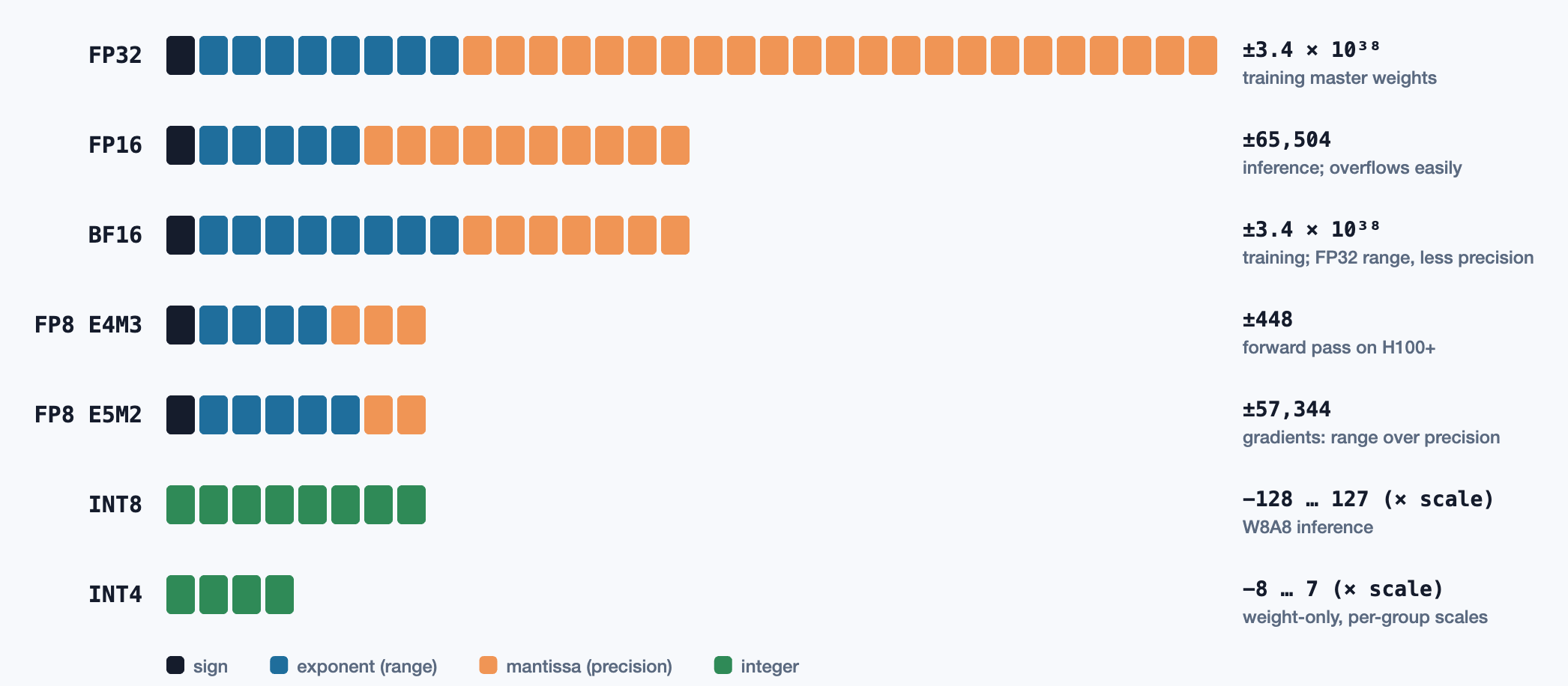
Floating-point formats spend bits on an exponent, so their precision is relative: fine near zero, coarse for large values. Integers have evenly spaced levels and rely on a separate scale to map them onto real values. Newer hardware blurs the line with block formats such as the OCP Microscaling (MX) formats and NVIDIA’s NVFP4. Small groups of low-bit values share one scale factor stored alongside them, giving integer-like density with float-like dynamic range.

Scales, zero points and groups

Uniform quantisation to b bits maps a real value x to an integer and back:

The scale s sets the step size, and the zero point z lets the grid be asymmetric. A symmetric scheme drops z and sets s = max|x| / (2^b−1 − 1). The crucial choice is granularity, meaning how many values share one scale:

• Per-tensor: one scale for the whole matrix. Cheap, and ruined by a single large value.
• Per-channel: one scale per output row of a weight matrix. The standard for INT8 weights.
• Per-group: one scale per block of, typically, 128 consecutive weights. This is what makes 4-bit weights work, at a cost of about 0.125–0.25 extra bits per weight for the scales.

Outliers break the naive approach

Weights are well-behaved: roughly bell-shaped, with few extremes. Activations are not. Dettmers et al. (LLM.int8(), 2022) found that once transformers pass roughly 6.7 billion parameters, a handful of hidden dimensions develop systematic outliers, values many times larger than the rest, and those dimensions carry information the model depends on. Quantise activations per tensor and the outliers set the scale: everything else is squeezed into a few levels near zero and effectively erased. LLM.int8() handled this by keeping the outlier dimensions in 16-bit and multiplying them separately (a mixed-precision decomposition). It worked, but the decomposition is slow.

SmoothQuant

SmoothQuant (Xiao et al., 2022) starts from an identity. For a linear layer Y = XW, any positive per-channel scaling can be moved from one side to the other:

Dividing the outlier channels of X by a large s_j shrinks them. Multiplying the corresponding rows of W by the same factor keeps the product unchanged. With α = 0.5, the activation and weight ranges for each channel end up equal. The difficulty is split between the two, where weights, which quantise easily, absorb their half. The scaled weights are computed once offline, and the activation scaling is folded into the preceding layer norm, so inference costs nothing extra.

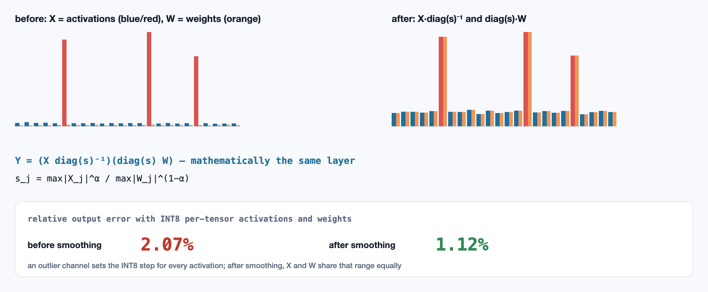
This made W8A8 (INT8 weights and activations) work for models such as OPT-175B, with up to 1.56× faster inference and half the memory, at almost no loss of accuracy.

GPTQ: second-order error correction

For weight-only quantisation to 3–4 bits, the question is which grid point each weight should go to. Rounding to the nearest one minimises the error in the weights. What matters is the error in the layer’s output on real inputs:

Inputs are correlated, so errors in different weights can cancel. If rounding pushed one weight up, nudging a correlated weight down can undo most of the effect on the output. GPTQ (Frantar et al., 2022) builds on Optimal Brain Surgeon: quantise one weight (column) at a time, then update all the not-yet-quantised weights to absorb the error, using the inverse Hessian H⁻¹ = (2XX^⊤)⁻¹:

Three engineering ideas made this practical at the scale of a 175B model:

• A fixed order. OBS picks the next weight greedily, which is expensive. GPTQ found that quantising columns in plain left-to-right order is almost as good, and then H⁻¹ is the same for every row of the matrix, so all rows are processed together.
• Cholesky. Repeatedly updating H⁻¹ is numerically unstable. Everything the algorithm needs is in the rows of the upper Cholesky factor of H⁻¹, computed once.
• Lazy batching. Updates are applied to blocks of 128 columns at a time, keeping the GPU busy with matrix multiplies instead of memory-bound vector updates.

The paper quantised OPT-175B and BLOOM-176B to 3–4 bits in about four GPU hours with little loss of perplexity, enough to run a 175B model on a single 80 GB A100.

AWQ: protect the salient channels

AWQ (Lin et al., 2023) starts from an observation: not all weights matter equally. Keeping just ~1% of weight channels, those that meet the largest activations, in full precision recovers most of the quantisation loss. Mixed precision is awkward for hardware, though, so AWQ protects those channels by scaling instead: multiply a salient input channel’s weights by s > 1 before quantising, and divide its activation by the same s. The weight’s relative rounding error shrinks, and the product is unchanged:

AWQ needs no backpropagation and no second-order information, only activation statistics. That makes it fast and less prone to overfitting the calibration set. It has become one of the standard 4-bit formats for serving, and won the best paper award at MLSys 2024.

Beyond weights

• KV cache. At long context the KV cache can outgrow the weights. KIVI quantises keys per channel and values per token to 2 bits, because keys have outlier channels and values don’t.
• QLoRA’s NF4. For fine-tuning, QLoRA stores the frozen base model in a 4-bit “NormalFloat” format whose levels are quantiles of a normal distribution, matching how weights are actually distributed, and trains LoRA adapters in 16-bit on top.
• FP8 training. Hopper-class GPUs train in FP8, using E4M3 for forward activations and weights and E5M2 for gradients, with per-tensor or per-block scales maintained during training.
• Rotations. Methods such as QuaRot and SpinQuant multiply by orthogonal matrices that spread outliers across all dimensions before quantising, the same trick FlashAttention-3 uses for FP8.

GPTQ in code

The full algorithm for one row, with its helpers. The figure above runs exactly this.

// GPTQ for one row of a weight matrix. X holds calibration inputs (n samples x d features).
// The same updates apply to every row at once in the real algorithm, since H is shared.
const quantise = (x: number, scale: number, levels = 7) => {
  const m = (levels - 1) / 2;
  return scale * Math.max(-m, Math.min(m, Math.round(x / scale)));
};

export function gptqRow(w: number[], X: number[][], scale: number, dampRatio = 0.01) {
  const d = w.length, n = X.length;
  // H = 2 X^T X / n: the Hessian of the squared output error with respect to w.
  const H = Array.from({ length: d }, (_, i) =>
    Array.from({ length: d }, (_, j) => (2 * X.reduce((s, x) => s + x[i] * x[j], 0)) / n));
  const damp = (dampRatio * H.reduce((s, row, i) => s + row[i], 0)) / d;
  H.forEach((row, i) => (row[i] += damp)); // keeps H invertible

  // Upper Cholesky factor of H^-1: row q carries the OBS update for column q,
  // with the columns before q already eliminated.
  const U = cholUpper(inverse(H));

  const q = w.slice(), out = new Array(d);
  for (let c = 0; c < d; c++) {
    out[c] = quantise(q[c], scale);
    const err = (q[c] - out[c]) / U[c][c];
    for (let j = c + 1; j < d; j++) q[j] -= err * U[c][j]; // compensate on the rest
  }
  return out;
}

// Plain helpers: Gauss-Jordan inverse and an upper Cholesky factor (A = U^T U).
function inverse(A: number[][]) {
  const n = A.length;
  const M = A.map((row, i) => [...row, ...row.map((_, j) => (i === j ? 1 : 0))]);
  for (let c = 0; c < n; c++) {
    let p = c;
    for (let r = c + 1; r < n; r++) if (Math.abs(M[r][c]) > Math.abs(M[p][c])) p = r;
    [M[c], M[p]] = [M[p], M[c]];
    const piv = M[c][c];
    for (let j = 0; j < 2 * n; j++) M[c][j] /= piv;
    for (let r = 0; r < n; r++) {
      if (r === c) continue;
      const f = M[r][c];
      for (let j = 0; j < 2 * n; j++) M[r][j] -= f * M[c][j];
    }
  }
  return M.map((row) => row.slice(n));
}

function cholUpper(A: number[][]) {
  const n = A.length, L = A.map(() => new Array(n).fill(0));
  for (let i = 0; i < n; i++)
    for (let j = 0; j <= i; j++) {
      let s = A[i][j];
      for (let k = 0; k < j; k++) s -= L[i][k] * L[j][k];
      L[i][j] = i === j ? Math.sqrt(s) : s / L[j][j];
    }
  return L[0].map((_, i) => L.map((row) => row[i])); // the transpose of L
}

References

1. Dettmers, T. et al. (2022). LLM.int8(): 8-bit Matrix Multiplication for Transformers at Scale. arXiv:2208.07339
2. Xiao, G. et al. (2022). SmoothQuant: Accurate and Efficient Post-Training Quantization for Large Language Models. arXiv:2211.10438
3. Frantar, E. et al. (2022). GPTQ: Accurate Post-Training Quantization for Generative Pre-trained Transformers. arXiv:2210.17323
4. Lin, J. et al. (2023). AWQ: Activation-aware Weight Quantization for LLM Compression and Acceleration. arXiv:2306.00978
5. Hassibi, B. & Stork, D. (1993). Second Order Derivatives for Network Pruning: Optimal Brain Surgeon. NeurIPS. proceedings.neurips.cc
6. Dettmers, T. et al. (2023). QLoRA: Efficient Finetuning of Quantized LLMs. arXiv:2305.14314
7. Liu, Z. et al. (2024). KIVI: A Tuning-Free Asymmetric 2bit Quantization for KV Cache. arXiv:2402.02750
8. Micikevicius, P. et al. (2022). FP8 Formats for Deep Learning. arXiv:2209.05433
9. Ashkboos, S. et al. (2024). QuaRot: Outlier-Free 4-Bit Inference in Rotated LLMs. arXiv:2404.00456