Mixture-of-Experts: sparse models, routing and the cost of balance

The largest open language models are no longer dense. DeepSeek-V3 has 671 billion parameters but uses only 37 billion of them for any given token. Mixtral 8x7B has 47 billion and uses 13. The trick is the Mixture-of-Experts layer: many parallel feed-forward networks, and a small router that sends each token to just a few of them. Capacity grows with the number of experts. Compute per token grows only with the number chosen.

It sounds like a free lunch, and it isn’t. Routers want to send everything to the same expert, experts overflow, and the experts end up on different GPUs, so tokens have to cross the network twice per layer. This article covers how the layer works, why it is hard to train, the balancing tricks that make it work, and what sparsity costs at serving time.

Why sparse

In a transformer, most parameters live in the feed-forward (FFN) blocks, roughly two thirds of the total. Every token passes through all of them. Scaling laws say quality keeps improving with parameters, but in a dense model every added parameter adds compute for every token, in training and in inference.

Conditional computation breaks that link: give the model many FFNs, but let each token use only a few. The idea is old (Jacobs et al., 1991), but it became practical for deep learning with Shazeer et al.’s sparsely-gated MoE in 2017, then GShard (2020), which scaled it to a 600B-parameter translation model, and the Switch Transformer (2021), which reported up to 7× faster pre-training than a dense T5 with the same compute per token.

The MoE layer

The layer replaces one FFN with E expert FFNs and a router, which is a single linear layer W_g producing one logit per expert. For a token with hidden state x:

Only the k selected experts run. Their outputs are mixed by the renormalised gate weights. Mixtral uses 8 experts with k = 2, the Switch Transformer used k = 1, and DeepSeek-V3 uses 256 routed experts with k = 8 plus one shared expert every token visits. Because the gate weights multiply the outputs, the router gets gradients through them and learns which experts suit which tokens. The hard top-k selection itself is not differentiable, which is the root of the trouble.

What do experts specialise in? Less than the name suggests. The Mixtral authors found no obvious alignment between experts and topics such as biology or philosophy. Routing correlated more with syntax and token type, and consecutive tokens often went to the same expert. Experts are a capacity mechanism, not a committee of specialists.

Router collapse and load balancing

Early in training, some expert is slightly better at random. The router sends it more tokens, so it trains more and gets better, so the router sends it even more. Left alone, this rich-get-richer loop collapses routing onto a few experts. The rest receive no tokens and no gradient, and the model degrades into a small dense one with wasted memory.

The standard fix is an auxiliary load-balancing loss. The Switch Transformer’s version is:

Here f_i is the fraction of tokens actually dispatched to expert i, and P_i is the average router probability for it. f is not differentiable but P is, so the gradient pushes probability away from experts that are receiving too many tokens. The sum is minimised at 1 when routing is uniform, and α ≈ 0.01 keeps it from overpowering the language-modelling loss. ST-MoE added a router z-loss, a penalty on the squared log-sum-exp of the router logits, which keeps them small and fixes a common source of training instability.

Auxiliary losses have a cost: they fight the main objective, and too much balancing hurts quality. DeepSeek-V3 replaced most of it with an auxiliary-loss-free scheme. Each expert gets a bias that is added to its score only when choosing the top-k. The gate weights still use the unbiased scores. After each training step, the bias of an overloaded expert is nudged down and that of an underloaded one nudged up. Balance is enforced by a controller rather than a gradient, so the language-modelling objective is left alone. The second half of Fig. 1 is that mechanism.

Capacity and dropped tokens

Hardware wants static shapes: each expert processes a fixed-size buffer. The buffer size is the expert capacity:

With a capacity factor of 1.0, a perfectly balanced batch exactly fills every expert. Any imbalance overflows someone. Overflowing assignments are dropped: that expert simply doesn’t process the token, and the token continues through the residual connection, as if this layer’s FFN had output zero for it. A factor of 1.25–2.0 trades memory and wasted compute on padding for fewer drops. Dropping is tolerable in training, since the gradient is just noisier, but at inference it means a token’s output depends on what else is in the batch, which is why many modern systems, DeepSeek-V3 among them, avoid dropping altogether.

Expert parallelism

A model with hundreds of experts doesn’t fit on one GPU, so experts are sharded across devices: expert parallelism. Attention layers are replicated or sharded as usual. At each MoE layer, every GPU has tokens that want experts living on other GPUs.

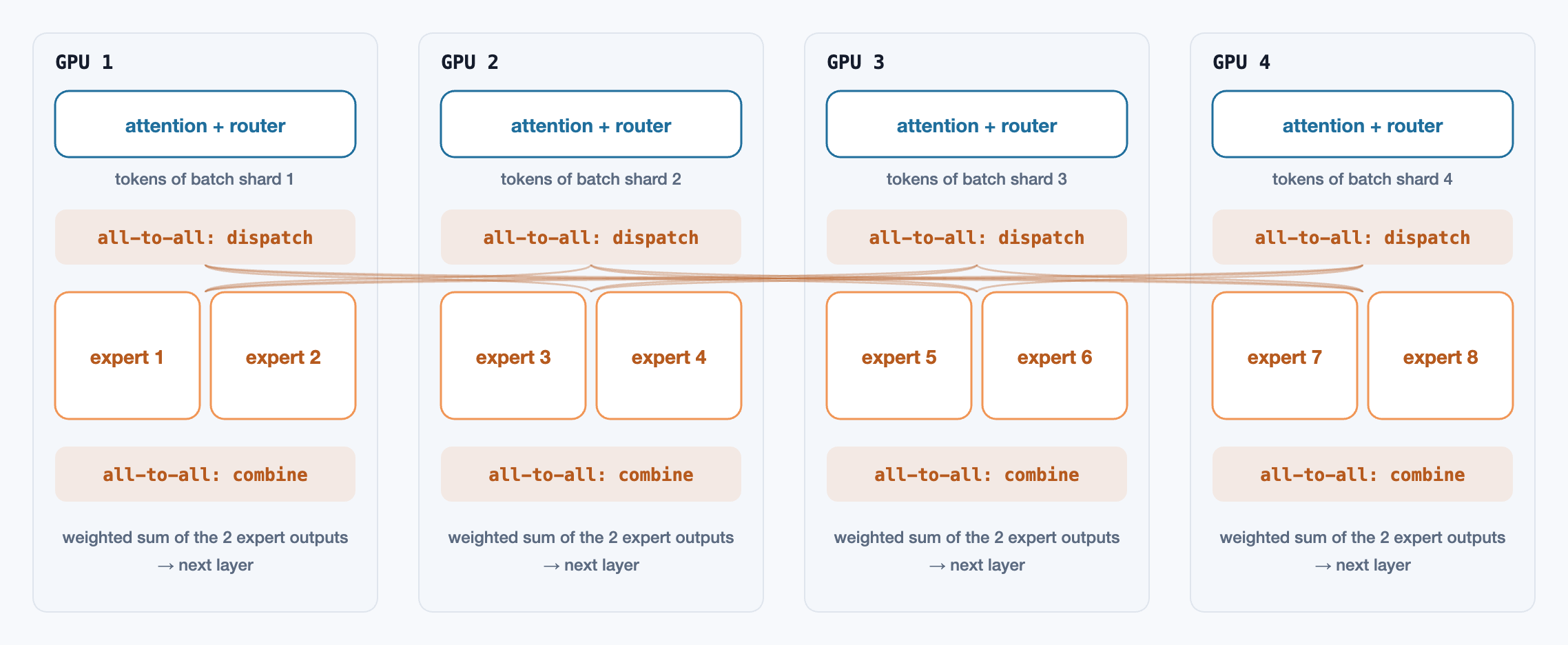
All-to-all is the most demanding collective operation there is: every device sends a different payload to every other device. Its cost scales with tokens × k × hidden size, and across nodes it runs over the slowest link in the cluster. Systems fight it in several ways: limiting how many nodes a token may route to (DeepSeek-V3 caps it at four), overlapping communication with computation, keeping popular experts replicated, and placing experts so that common routes stay inside a node.

Total vs active parameters

An MoE model has two parameter counts, and they measure different things. Total parameters determine memory: every expert must be resident somewhere. Active parameters determine compute per token: only the chosen experts run.

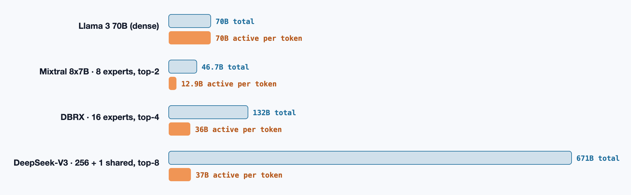
The gap has consequences that are easy to miss:

• Memory doesn’t shrink. Serving Mixtral needs the memory of a 47B model, not a 13B one. MoE trades memory for compute, which is the right trade in a large cluster and the wrong one on a laptop.
• Small batches lose the advantage. Decoding is memory-bound. With many tokens in a batch, different tokens hit different experts, so nearly all expert weights are read every step anyway. MoE inference shines at high throughput, where weight reads are amortised across many tokens.
• Quality per active parameter is high, but not per total parameter. An MoE usually beats a dense model with the same active parameters and loses to a dense model with the same total parameters.

Modern designs

• Fine-grained experts (DeepSeekMoE). Split each expert into several smaller ones and activate proportionally more. The number of possible expert combinations explodes, and specialisation becomes sharper.
• Shared experts. One or a few experts that every token uses, holding common knowledge so the routed experts don’t all need to duplicate it.
• Upcycling. Initialise every expert as a copy of a trained dense FFN, then continue training as an MoE. This is cheaper than training sparse from scratch (Komatsuzaki et al., 2022).
• Fine-tuning care. MoE models overfit more easily in fine-tuning, and routers can shift abruptly. Common practice is to freeze or regularise the router, or use a higher dropout in experts.

A layer in code

The forward pass of one layer: router softmax, top-k selection, renormalised gate weights, capacity enforcement, and the Switch balance loss.

// One MoE layer's forward pass for a batch of tokens, with top-k gating and capacity.
type Vec = number[];
type Expert = (x: Vec) => Vec; // a feed-forward block

const softmax = (v: Vec) => {
  const m = Math.max(...v), e = v.map((x) => Math.exp(x - m)), z = e.reduce((a, b) => a + b, 0);
  return e.map((x) => x / z);
};
const dot = (a: Vec, b: Vec) => a.reduce((s, x, i) => s + x * b[i], 0);

export function moeLayer(tokens: Vec[], Wg: Vec[], experts: Expert[], k = 2, capacityFactor = 1.25) {
  const T = tokens.length, E = experts.length;
  const capacity = Math.ceil((capacityFactor * T * k) / E);
  const load = new Array(E).fill(0);
  const f = new Array(E).fill(0), P = new Array(E).fill(0); // for the balance loss

  const out = tokens.map((x) => {
    const probs = softmax(Wg.map((w) => dot(w, x)));  // router: one logit per expert
    probs.forEach((p, e) => (P[e] += p / T));
    const top = probs.map((p, e) => [p, e]).sort((a, b) => b[0] - a[0]).slice(0, k);
    const norm = top.reduce((s, [p]) => s + p, 0);    // renormalise over the chosen k

    const y = new Array(x.length).fill(0);
    for (const [p, e] of top) {
      f[e] += 1 / (T * k);
      if (load[e] >= capacity) continue;               // overflow: this expert is full
      load[e]++;
      const h = experts[e](x);
      for (let i = 0; i < y.length; i++) y[i] += (p / norm) * h[i];
    }
    // The residual connection outside this function carries x through regardless,
    // so a token whose experts were all full simply passes the layer unchanged.
    return y;
  });

  // Switch-style auxiliary loss: E * sum_i f_i * P_i, minimised (= 1) at uniform routing.
  const balanceLoss = E * f.reduce((s, fi, e) => s + fi * P[e], 0);
  return { out, balanceLoss };
}

References

1. Shazeer, N. et al. (2017). Outrageously Large Neural Networks: The Sparsely-Gated Mixture-of-Experts Layer. arXiv:1701.06538
2. Lepikhin, D. et al. (2020). GShard: Scaling Giant Models with Conditional Computation and Automatic Sharding. arXiv:2006.16668
3. Fedus, W., Zoph, B. & Shazeer, N. (2021). Switch Transformers: Scaling to Trillion Parameter Models with Simple and Efficient Sparsity. arXiv:2101.03961
4. Zoph, B. et al. (2022). ST-MoE: Designing Stable and Transferable Sparse Expert Models. arXiv:2202.08906
5. Zhou, Y. et al. (2022). Mixture-of-Experts with Expert Choice Routing. arXiv:2202.09368
6. Komatsuzaki, A. et al. (2022). Sparse Upcycling: Training Mixture-of-Experts from Dense Checkpoints. arXiv:2212.05055
7. Jiang, A. Q. et al. (2024). Mixtral of Experts. arXiv:2401.04088
8. Dai, D. et al. (2024). DeepSeekMoE: Towards Ultimate Expert Specialization in Mixture-of-Experts Language Models. arXiv:2401.06066
9. DeepSeek-AI (2024). DeepSeek-V3 Technical Report. arXiv:2412.19437
10. Jacobs, R. A., Jordan, M. I., Nowlan, S. J. & Hinton, G. E. (1991). Adaptive Mixtures of Local Experts. Neural Computation. doi:10.1162/neco.1991.3.1.79