How the query planner picks a join

The same SQL can run in a millisecond or an hour, depending on choices you never wrote down: which table to read first, how to match rows between tables, and whether to use an index at all. The query planner makes those choices from estimates, and when a query is slow it is usually because one of those estimates was badly wrong, not because the database is slow.

This article covers how a query becomes a plan tree, the three join algorithms and when each wins, how the planner estimates row counts and where that goes wrong, join order, reading EXPLAIN ANALYZE, queries the planner interprets differently from how they read, and generic plans for prepared statements. Examples use Postgres; the ideas apply to every cost-based optimiser. Choosing indexes is covered separately, in the article on database indexes.

From SQL to a plan tree

SQL says what result you want, not how to compute it. The database parses the query, rewrites it (expanding views, inlining simple subqueries), then the planner considers the ways it could be executed, estimates the cost of each, and keeps the cheapest. The result is a tree of operators: scans at the leaves, then joins, sorts, aggregates and limits above them.

Execution pulls rows up the tree. Each node asks its children for the next row, does its work, and hands rows to its parent. That is why a LIMIT 10 at the top can stop a scan underneath after ten rows, and why one node producing far more rows than expected makes every node above it slow too.

Nested loop, hash and merge joins

Every two-table join in the plan uses one of three algorithms. They all return the same rows; they differ in how the work grows with the size of each side.

An everyday version of the problem: you have a stack of parcels and a list of addresses, and you need to pair each parcel with its address. With three parcels and an alphabetical address book, you look each one up: that is a nested loop. With ten thousand parcels, looking each one up is slow, so you first sort the address list into labelled pigeonholes and then drop each parcel into the right one: that is a hash join. If the parcels and the addresses both arrived already sorted by name, you walk down both piles at once: that is a merge join. None of these is the best method in general. Which one wins depends on how many parcels there are and how they arrived.

• Nested loop. For each row of the outer input, look up matching rows in the inner input. With an index on the inner join column, each lookup is a few page reads, so the cost is roughly the outer row count times one index probe. Unbeatable when the outer side is small; disastrous when it is large. It is also the only algorithm that handles arbitrary join conditions, such as ranges or LIKE.
• Hash join. Read the smaller input and build an in-memory hash table on the join key, then read the larger input once and probe the table for each row. The cost is about one pass over each side, regardless of indexes. It only works for equality, and the hash table must fit in work_mem (times hash_mem_multiplier); otherwise it is split into batches written to disk, which EXPLAIN shows as Batches greater than 1.
• Merge join. Sort both inputs on the join key, or read them in order from indexes, and walk them forward together. Cheap if the inputs are already sorted, and it needs little memory, but explicit sorts of large inputs can cost more than hashing.

The pattern in practice: nested loops dominate OLTP queries that touch a few rows through indexes; hash joins dominate reporting queries that join large fractions of tables; merge joins appear when both sides come out of an index in key order, or when the result must be sorted anyway.

Everything depends on row estimates

The planner can only choose well if it knows how many rows each step will produce. It estimates that from statistics that ANALYZE collects by sampling each table: the fraction of nulls, the number of distinct values, the most common values with their frequencies, and a histogram of the rest. For WHERE status = 'paid', it looks up how common paid is and multiplies by the table’s row count.

For several conditions, it multiplies their selectivities, assuming the columns are independent. That assumption is the most common cause of bad plans. City and country, product and category, state and zip code are all strongly correlated: knowing the city tells you the country. Multiplying underestimates the result, often by orders of magnitude, and an underestimate is exactly what makes a nested loop look cheap.

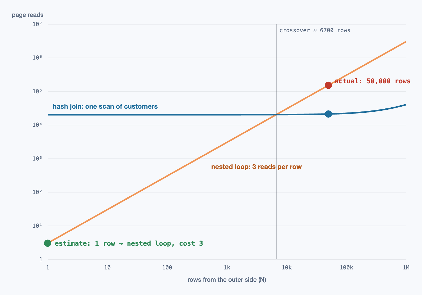
Other common sources of bad estimates:

• Stale statistics after a bulk load or a big delete, before autovacuum has run ANALYZE. Run it yourself after large data changes.
• Expressions and functions the planner can’t see into, such as WHERE lower(email) = … or a user-defined function, which get a default selectivity guess. An expression index also gathers statistics on the expression.
• Skew beyond the most-common-values list: one tenant with 40% of the rows looks like an average tenant if it isn’t in the sample’s top values. Raising the column’s statistics target helps.
• Errors compounding through joins. Each join multiplies estimates together, so a 10× error at the bottom of a five-way join can be 10,000× at the top.

Join order

With more than two tables, the planner also chooses the order in which to join them, and the number of possible orders grows factorially. Postgres searches the orders exhaustively, with dynamic programming, up to geqo_threshold (12 tables by default), and falls back to a genetic algorithm above that. It also stops reordering explicit JOINs beyond join_collapse_limit (8), keeping the written order instead.

The goal of a good order is to shrink intermediate results early: apply the most selective filters and joins first, so later joins handle fewer rows. That is another place where estimates decide everything. For queries that join a dozen or more tables, generated by ORMs or reporting tools, the written order starts to matter, and splitting the query or materialising a small intermediate result can help.

Reading EXPLAIN ANALYZE

EXPLAIN shows the chosen plan with estimates. EXPLAIN (ANALYZE, BUFFERS) runs the query and adds what actually happened at each node. Read it from the innermost nodes outwards, and look for these in order:

1. Estimated rows against actual rows. The planner’s rows= next to actual … rows=. A gap of 10× is worth noting; 100× usually explains the whole plan. Find the lowest node where the gap appears: that is where the misestimate starts.
2. loops. The actual rows and time are per loop. An inner index scan showing 10 rows and 0.05 ms with loops=50000 really produced 500,000 rows and took 2.5 seconds.
3. Buffers. shared hit is pages found in cache, read is pages read from the OS or disk. Pages, not milliseconds, are the stable measure of how much work a plan does: timing depends on what was cached.
4. Rows Removed by Filter. A scan that reads a million rows to return a thousand is doing the filtering the wrong way round; an index might help.
5. Spills. Batches greater than 1 on a hash, or Sort Method: external merge Disk, mean the operation ran out of work_mem.

Queries the planner reads differently

• NOT IN with a subquery returns no rows if the subquery produces a single NULL, and Postgres can’t turn it into an efficient anti-join. NOT EXISTS means what people usually intend and is planned as an anti-join.
• OR across columns (WHERE a = 1 OR b = 2) often prevents a single index scan. Postgres can combine two indexes with a BitmapOr; otherwise, a UNION of two indexed queries may be faster.
• CTEs are inlined into the main query since Postgres 12, unless they are referenced twice or marked MATERIALIZED. Older advice to use a CTE as an “optimisation fence”, or to avoid CTEs because they were one, no longer applies by default.
• Correlated subqueries in the SELECT list run once per row: a hidden nested loop. Rewriting them as a join or a LATERAL join gives the planner the choice back.
• OFFSET pagination reads and discards every skipped row. Page 1,000 of 20 reads 20,020 rows. Keyset pagination (WHERE id > $last ORDER BY id LIMIT 20) reads 20.

Prepared statements and generic plans

A prepared statement, which most drivers and ORMs use, can be planned once for any parameter values. Postgres plans the first five executions with the actual values (custom plans), then compares their average cost with a generic plan that ignores the values, and switches to the generic plan if it isn’t estimated to be worse.

With skewed data this produces a classic production mystery: a query that is fast in psql and slow from the application. The generic plan was chosen from typical values and is terrible for the one large tenant. plan_cache_mode = force_custom_plan, set for the role or the session, makes Postgres replan with real values every time, at the cost of planning on each execution. Check whether you are using a generic plan by running EXPLAIN EXECUTE on the prepared statement more than five times.

Fixing a bad plan

In rough order of preference:

1. Fix the estimate. ANALYZE; raise the statistics target for skewed columns; create extended statistics (CREATE STATISTICS) for correlated columns. The planner then chooses well for this query and every other query that touches the same columns.
2. Give it a better option. An index that matches the join and filter, or a covering index that avoids heap fetches.
3. Rewrite the query into a form the planner handles well: NOT EXISTS, keyset pagination, a join instead of a correlated subquery, or splitting a huge query.
4. Adjust settings narrowly. work_mem for a reporting role so hashes and sorts stay in memory; random_page_cost closer to 1.1 on SSDs, so index scans aren’t overpriced.
5. Force it, as a last resort. Postgres has no built-in hints. Disabling a join type for a session (SET enable_nestloop = off) or the pg_hint_plan extension pin a plan, but a pinned plan doesn’t adapt when the data changes.

Plans also change on their own when statistics change, which is how a query that was fine for a year becomes slow overnight. Logging slow plans automatically with auto_explain catches the plan at the moment it went wrong, instead of an hour later when it might be different again.

A misestimate, found and fixed

A query whose correlated filter is underestimated by a factor of a thousand, the nested loop that results, the extended statistics that correct the estimate, and the hash join the planner picks once it knows the real numbers.

-- Orders from customers in Paris placed this month, with the customer's name.
EXPLAIN (ANALYZE, BUFFERS)
SELECT o.id, o.total, c.name
FROM customers c
JOIN orders o ON o.customer_id = c.id
WHERE c.city = 'Paris' AND c.country = 'FR'
  AND o.created_at >= date_trunc('month', now());

-- Abridged output before the fix. Read estimated rows against actual rows:
--
-- Nested Loop  (rows=12) (actual time=0.9..2843.1 rows=48210 loops=1)
--   Buffers: shared hit=81240 read=64117
--   ->  Seq Scan on customers c  (rows=3) (actual rows=4870 loops=1)
--         Filter: ((city = 'Paris') AND (country = 'FR'))
--         Rows Removed by Filter: 995130
--   ->  Index Scan using orders_customer_id_idx on orders o
--         (rows=4) (actual rows=10 loops=4870)
--         Filter: (created_at >= date_trunc('month', now()))
--
-- The planner expected 3 Paris customers, because it multiplied the selectivity
-- of city by the selectivity of country as if they were independent. It got 4,870,
-- so the inner index scan ran 4,870 times instead of 3.

-- Tell the planner the columns are related, and refresh the statistics.
CREATE STATISTICS customers_city_country (dependencies, ndistinct, mcv)
  ON city, country FROM customers;
ANALYZE customers;

-- After: the estimate is close, and the plan changes to match.
--
-- Hash Join  (rows=46800) (actual time=41.2..212.7 rows=48210 loops=1)
--   Hash Cond: (o.customer_id = c.id)
--   ->  Index Scan using orders_created_at_idx on orders o  (rows=611000) ...
--   ->  Hash  (rows=4910) (actual rows=4870 loops=1)
--         Buckets: 8192  Batches: 1  Memory Usage: 402kB
--         ->  Seq Scan on customers c  (rows=4910) (actual rows=4870 loops=1)

-- Is a hash spilling to disk? Batches > 1 means yes. Raise memory for this session only.
SET work_mem = '64MB';

References

1. Selinger, P. G. et al. (1979). Access Path Selection in a Relational Database Management System. SIGMOD. doi:10.1145/582095.582099
2. Graefe, G. (1993). Query Evaluation Techniques for Large Databases. ACM Computing Surveys. doi:10.1145/152610.152611
3. Leis, V. et al. (2015). How Good Are Query Optimizers, Really? VLDB. vldb.org
4. PostgreSQL Documentation. Using EXPLAIN, Statistics Used by the Planner and CREATE STATISTICS. postgresql.org/docs/current/using-explain.html
5. PostgreSQL Documentation. PREPARE (custom and generic plans, plan_cache_mode). postgresql.org/docs
6. Winand, M. Use The Index, Luke: The Join Operation. use-the-index-luke.com/sql/join