How database indexes really work

Most slow queries are fixed with an index, and most bad indexes come from treating them as a magic switch: add one on the column in the WHERE clause and hope. An index is a data structure with a specific shape, and it can only help queries that fit that shape. Once you can picture it, choosing indexes, reading query plans and predicting the planner’s decisions all become mechanical.

This article covers how a B-tree index is laid out and traversed, why the planner sometimes ignores a perfectly good index, how column order decides which queries a composite index can serve, covering, partial and expression indexes, and what each index costs on every write. Examples use Postgres; MySQL’s InnoDB differs in the places noted.

What a B-tree index is

The default index in Postgres, MySQL, SQL Server and Oracle is a B+tree: a balanced tree of fixed-size pages, 8 KB in Postgres and 16 KB in InnoDB. Leaf pages hold the indexed values in sorted order, each with a pointer to its row, and are linked to their neighbours so a scan can walk sideways. Internal pages hold only separator keys that route a search to the right child.

Because each page holds hundreds of entries, the tree is very shallow. With a fan-out of a few hundred, three levels cover tens of millions of rows and four cover billions. The top levels are read so often that they stay in memory, so a lookup typically costs one or two actual disk reads. That is where the B-tree’s O(log n) comes from, with a very large base. (Why some databases use LSM-trees instead, trading read cost for write throughput, is covered in the LSM-tree article.)

Seek, scan, fetch

Using an index for a range query is three separate steps, and each has its own cost:

1. Seek. Descend from the root to the first leaf entry that matches: one page per level.
2. Scan. Walk along the leaves, in key order, until the entries stop matching. Leaf entries are packed together, so this is cheap.
3. Fetch. For each matching entry, follow its pointer to the row in the table to read the columns the index doesn’t hold. Rows with neighbouring keys are rarely on neighbouring pages, so this step is random I/O, one page per row in the worst case.

The fetch step is usually where the time goes. Postgres shows the three ways of handling it in EXPLAIN:

• Index Scan: fetch each row as its entry is found. Good for a handful of rows.
• Bitmap Heap Scan: collect all matching row locations first, sort them by page, then read each page once in physical order. Good for thousands of rows spread across the table.
• Index Only Scan: answer from the index alone, skipping the table. Only possible when the index holds every column the query needs (and, in Postgres, when the visibility map shows the pages are all-visible, which VACUUM maintains).

When the planner ignores your index

The query planner estimates the cost of every reasonable plan and picks the cheapest. A sequential scan reads the whole table, but in large sequential chunks; an index scan reads less, but randomly. If a query matches a large fraction of the table, often more than a few percent, reading everything sequentially is cheaper than thousands of random fetches, and the planner is right to ignore the index.

When it ignores an index it shouldn’t, the cause is usually one of these:

• The column is wrapped in an expression. WHERE lower(email) = $1 or WHERE created_at::date = $1 can’t use an index on the bare column, because the index is sorted by the column, not by the expression. Rewrite the condition as a range on the column, or index the expression.
• A type mismatch. Comparing a text column to a number, or a timestamp to a timestamptz, can force a cast on the column side.
• Pattern matching. LIKE 'abc%' can use a B-tree (in Postgres, with the C collation or a text_pattern_ops index); LIKE '%abc' can’t, because nothing about the sort order helps. Use a trigram index (pg_trgm) for substring search.
• Wrong row estimates. The planner works from sampled statistics, and when they are stale or columns are correlated it can misjudge how many rows match by orders of magnitude. How estimates are made, how they go wrong, and how to read EXPLAIN (ANALYZE, BUFFERS) to spot it are covered in the article on query planning.

Composite indexes and column order

An index on several columns is sorted by the first column, then by the second within equal values of the first, and so on, like a phone book sorted by surname, then first name. That sort order decides which queries it can serve:

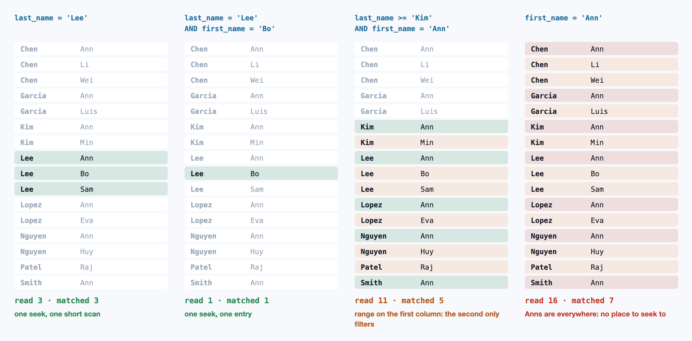
The rules that fall out of this:

• A query must constrain a leading prefix. An index on (a, b, c) serves queries on a, on a and b, and on all three. It can’t seek for a query on b alone. (Some databases can “skip scan” over a few distinct leading values, but don’t design around it.)
• Equality columns first, then one range column. After a range condition on a column, the index can no longer narrow by the columns that follow; they are only checked entry by entry. Put the columns tested with = first and the range or sort column last.
• Order matches ORDER BY for free. If the index order matches the query’s sort, for example (customer_id, created_at DESC) for “this customer’s orders, newest first”, the database reads rows already sorted and can stop after the LIMIT. That turns a sort of thousands of rows into reading twenty.
• One composite index often replaces several single-column ones. An index on (a, b) already serves queries on a alone, so a separate index on a is usually redundant.

The old advice to put the most selective column first is mostly wrong. What matters is which columns your queries test with equality, and which one they sort or range over.

Covering indexes

If the index contains every column a query reads, the fetch step disappears. Postgres 11 and later can add non-key columns to the leaves with INCLUDE: they are stored but not sorted, so they don’t change which queries the index can seek. SQL Server has the same syntax; in MySQL you append the columns to the key.

Covering indexes are the biggest single win for hot read paths, especially queries that return many rows. The cost is a larger index. Covering every column of a wide table just builds a second copy of it.

Partial and expression indexes

• Partial indexes index only the rows matching a condition: CREATE INDEX … WHERE status = 'pending'. If 1% of orders are pending and that is all the worker queries for, the index is a hundredth of the size and stays in memory. They are also how you enforce conditional uniqueness, such as one active subscription per user.
• Expression indexes index the result of an expression: ON users (lower(email)). The query must use the same expression to benefit.
• Other index types exist for queries B-trees can’t answer: GIN for arrays, JSONB and full-text search; GiST for ranges and geometry; BRIN for huge append-only tables where values correlate with physical order, such as timestamps in a log.

Clustered tables and primary keys

In Postgres, a table is a heap: rows sit wherever they were written, and every index, including the primary key, points into it. In MySQL’s InnoDB the table is a B+tree, ordered by the primary key, with the rows stored in its leaves. Two consequences for InnoDB:

• A secondary index stores the primary key as its pointer, so a lookup through it is two tree descents: the secondary index, then the primary key. A wide primary key also makes every secondary index wider.
• Random primary keys, such as UUIDv4, insert into random leaf pages, causing page splits, poor cache locality and bloated indexes. Sequential or time-ordered keys (auto-increment, or UUIDv7) append to the right edge of the tree. The same locality argument applies to Postgres indexes on random UUIDs, though less severely.

What every index costs

Indexes aren’t free. Every INSERT updates every index on the table, and every UPDATE that changes an indexed column updates that index. In Postgres, an update that touches no indexed column can be done as a cheap heap-only tuple (HOT) update; adding an index on a frequently updated column removes that optimisation for every update of it. Indexes also take memory: an index the hot path needs competes for cache with the data itself.

Indexes for a real query

A typical hot query, the index that serves it with an Index Only Scan and no sort, a partial alternative, how to confirm the plan, and how to find indexes that are only costing you writes.

-- The query: one customer's recent paid orders, newest first, with their totals.
SELECT id, created_at, total
FROM orders
WHERE customer_id = $1 AND status = 'paid' AND created_at >= now() - interval '90 days'
ORDER BY created_at DESC
LIMIT 20;

-- Equality columns first, the range/sort column last, and the selected column
-- carried in the leaf so the table is never visited: an Index Only Scan, no sort.
CREATE INDEX CONCURRENTLY orders_customer_paid_recent
  ON orders (customer_id, status, created_at DESC)
  INCLUDE (total);

-- If almost every query wants status = 'paid', a partial index is smaller still.
CREATE INDEX CONCURRENTLY orders_customer_paid
  ON orders (customer_id, created_at DESC)
  INCLUDE (total)
  WHERE status = 'paid';

-- Check what the planner actually does, with real timings and buffer counts.
EXPLAIN (ANALYZE, BUFFERS)
SELECT id, created_at, total FROM orders
WHERE customer_id = 42 AND status = 'paid' AND created_at >= now() - interval '90 days'
ORDER BY created_at DESC LIMIT 20;

-- Indexes nobody has used since statistics were last reset: candidates to drop.
SELECT relname AS table_name, indexrelname AS index_name, idx_scan,
       pg_size_pretty(pg_relation_size(indexrelid)) AS size
FROM pg_stat_user_indexes
WHERE idx_scan = 0
ORDER BY pg_relation_size(indexrelid) DESC;

References

1. Bayer, R. & McCreight, E. (1972). Organization and Maintenance of Large Ordered Indexes. Acta Informatica. doi:10.1007/BF00288683
2. Comer, D. (1979). The Ubiquitous B-Tree. ACM Computing Surveys. doi:10.1145/356770.356776
3. Winand, M. Use The Index, Luke: A Guide to Database Performance for Developers. use-the-index-luke.com
4. PostgreSQL Documentation. Chapter 11: Indexes and Using EXPLAIN. postgresql.org/docs/current/indexes.html
5. MySQL Reference Manual. Clustered and Secondary Indexes. dev.mysql.com
6. Petrov, A. (2019). Database Internals, ch. 2–4: B-Tree Basics and Implementation. O’Reilly. oreilly.com