Cell Culture Petri Dish Classification

Ting Tang

27 April 2026

1Task

Petri dish images are classified into 16 classes (a–q, excluding j). Three approaches are compared, each with two architectures:

A1. Scratch CNNs
- A1a. PowerfulCNN — residual network with CBAM attention
- A1b. SE-ResNet50 — ResNet50 with squeeze-and-excitation bottlenecks
A2. Fine-tuned Backbones
- A2a. Fine-tuned ConvNeXt-Small
- A2b. Fine-tuned Swin-T
A3. Embeddings + SVM
- A3a. ConvNeXt-Small embeddings + SVM
- A3b. Swin-T embeddings + SVM

2Dataset

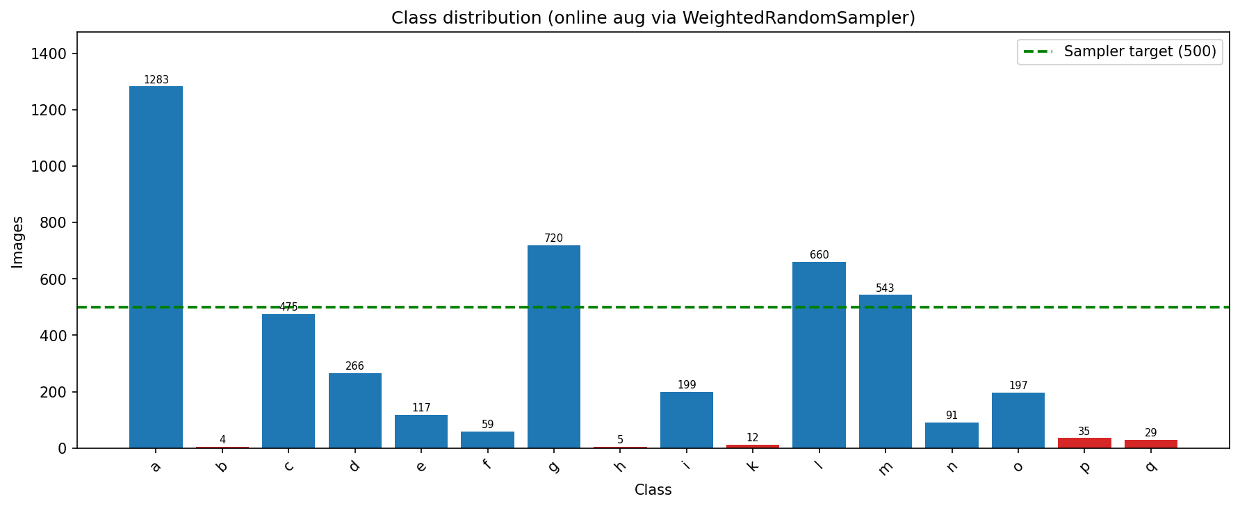
The dataset contains 4 695 labelled images across 16 classes (a–q, excluding j), supplemented by unlabelled test images. The dataset is severely imbalanced: class a dominates with 1 283 images while b has only 4, a raw imbalance ratio 1283/4 = 320×. The class distribution is shown in Figure 1.

A stratified 80/20 split yields 3 756 training samples and 939 held-out test samples.

Bar chart of images per class, from 1,283 down to 4 — Figure 1: Red bars indicate rare classes with fewer than 50 samples; the green dashed line marks the per-class target count (500) used by WeightedRandomSampler.

3Preprocessing Pipeline

3.1Stage 1 — YOLOv8-seg Dish Cropping

Each raw image is processed by a YOLOv8-nano-seg model [5] fine-tuned on 128 labelme-annotated petri dish images. Selected the highest-confidence segmentation mask; pixels outside the mask are set to white; the result is tight-cropped to the mask bounding box and resized to 320×320. If no mask is detected, the full image is used unchanged (Listing 1).

Listing 1: Stage 1 dish cropping: the highest-confidence YOLOv8-seg mask is kept, everything outside it set to white, and the result tight-cropped to the mask and resized to 320×320.

def crop_dish(img: np.ndarray, seg: YOLO) -> np.ndarray:
    # Stage 1: isolate the dish with the fine-tuned YOLOv8-nano-seg model.
    r = seg(img, verbose=False)[0]
    if r.masks is None:
        return img                              # no dish found: pass through
    best = int(r.boxes.conf.argmax())           # highest-confidence mask
    h, w = img.shape[:2]
    mask = cv2.resize(r.masks.data[best].cpu().numpy(), (w, h)) > 0.5
    img = np.where(mask[..., None], img, 255)   # background -> white
    ys, xs = np.nonzero(mask)
    img = img[ys.min():ys.max() + 1, xs.min():xs.max() + 1]
    return cv2.resize(img, (320, 320))

3.2Stage 2 — Colour Normalisation and ROI Refinement

On the YOLOv8-cropped images, four sequential corrections are applied:

Hough-circle ROI extraction. A Gaussian-blurred (11×11, σ = 2) greyscale image is passed to the gradient Hough transform (dp = 1.2, param₁ = 70, param₂ = 35, r ∈ [0.28, 0.62]⋅min(H, W)). The detected disc is expanded by 6% (r ← 1.06 r), masked to an ellipse (background = 128), and resized to 320×320. If no circle is found the image is passed through unchanged.
CLAHE [12] on the L^∗ channel of L^∗a^∗b^∗ space (clip limit 2.0, tile grid 8×8) enhances local contrast while preserving chrominance.

Grey-world white balance. Per-channel means over non-saturated pixels (intensity ∈ (10, 245)) are normalised to remove inter-session colour casts. For each channel c:
μ = 13 Σ_c μ_c, I_c ← clip(I_c ⋅ μ/μ_c, 0, 255).
(1)
Non-local means denoising [1] suppresses JPEG artefacts (h = 4, patch 7, window 21).

The two-stage output is a 320×320 RGB image; Listing 2 gives the code, and representative crops are shown in Figure 2.

Listing 2: Stage 2 on the cropped image: Hough-circle ROI refinement, CLAHE on the L^∗ channel, grey-world white balance over non-saturated pixels (Eq. 1), and non-local means denoising.

def normalise(img: np.ndarray) -> np.ndarray:
    # 1. Hough-circle ROI: expand the disc by 6%, mask to an ellipse.
    s = min(img.shape[:2])
    grey = cv2.GaussianBlur(cv2.cvtColor(img, cv2.COLOR_RGB2GRAY), (11, 11), 2)
    c = cv2.HoughCircles(grey, cv2.HOUGH_GRADIENT, dp=1.2, minDist=s,
                         param1=70, param2=35,
                         minRadius=int(0.28 * s), maxRadius=int(0.62 * s))
    if c is not None:
        x, y, r = c[0, 0]
        img = ellipse_roi(img, (x, y), 1.06 * r, fill=128, size=320)

    # 2. CLAHE on L* only, so chrominance is untouched.
    lab = cv2.cvtColor(img, cv2.COLOR_RGB2LAB)
    clahe = cv2.createCLAHE(clipLimit=2.0, tileGridSize=(8, 8))
    lab[..., 0] = clahe.apply(lab[..., 0])
    img = cv2.cvtColor(lab, cv2.COLOR_LAB2RGB)

    # 3. Grey-world white balance over non-saturated pixels.
    f = img.astype(np.float32)
    ok = (f.mean(-1) > 10) & (f.mean(-1) < 245)
    mu = f[ok].mean(axis=0)                     # per-channel means
    img = np.clip(f * mu.mean() / mu, 0, 255).astype(np.uint8)

    # 4. Non-local means against JPEG artefacts.
    return cv2.fastNlMeansDenoisingColored(img, None, h=4, hColor=4,
                                           templateWindowSize=7,
                                           searchWindowSize=21)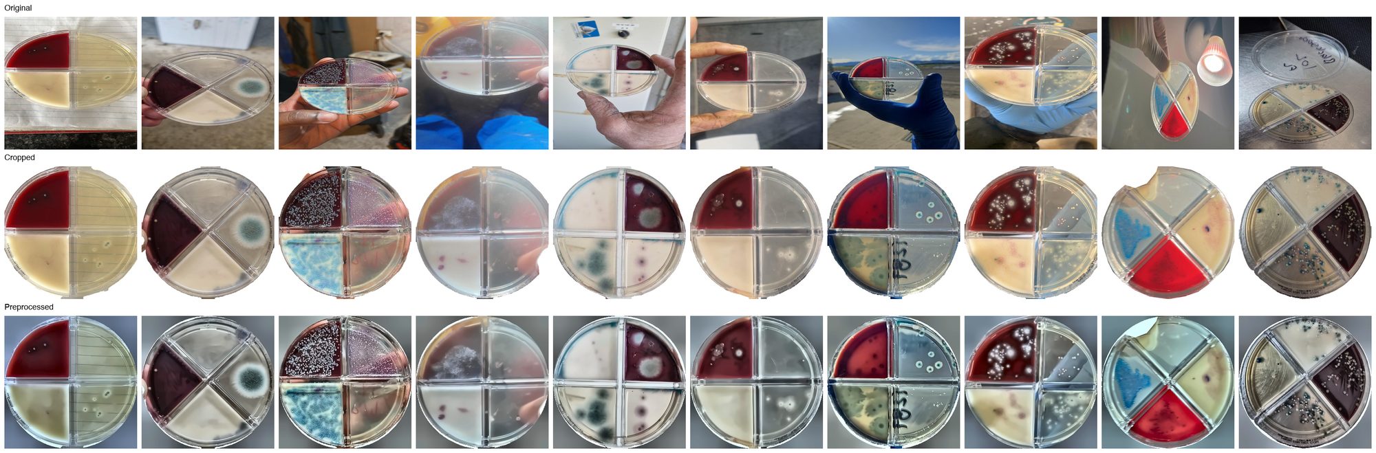

Three rows of petri dish photographs: raw, cropped, and colour-normalised — Figure 2: Representative preprocessing outputs for selected classes, one column per sample. **Top row:** the raw image. **Middle row:** after Stage 1 (YOLOv8-seg crop, background set to white, resized to 320×320). **Bottom row:** after Stage 2 (Hough-circle ROI extraction, CLAHE contrast enhancement, grey-world white balance, and NL-means denoising). Stage 2 visibly sharpens colony boundaries and reduces inter-session colour cast.

4Shared Training Infrastructure

4.1Data Split and Class Balancing

The 3 756 training originals are loaded with WeightedRandomSampler, drawing 500×16 = 8,000 samples per epoch with weight w^c = 500/n^c, equalising class frequency without duplicating validation data.

4.2Online Data Augmentation

Table 1 lists all transforms; fine-tuned backbones use wider rotation and crop variance and additionally apply RandomErasing.

Table 1: Online data augmentation parameters.

Transform	Parameter	Scratch CNNs (A1)	Fine-Tuned Backbones (A2)
RandomHorizontalFlip	p	0.5	0.5
RandomVerticalFlip	p	0.5	0.5
RandomRotation	degrees	±30°	±90°
RandomResizedCrop	scale, ratio	[0.9, 1.0], [0.95, 1.15]	[0.75, 1.0], [0.9, 1.1]
ColorJitter	b/c/s/h	0.20/0.20/0.15/0.03	0.30/0.30/0.20/0.05
RandomGrayscale	p	0.05	0.05
RandomAutocontrast	p	0.20	0.25
RandomAdjustSharpness	p	0.25	0.25
RandomErasing	p, scale	—	0.20, [0.02, 0.15]

4.3Focal Loss

Focal Loss [6] down-weights easy examples to keep the gradient signal focused on hard minority-class boundaries:

ℒ_focal(p, y) = −(1 − p_y)^γ log p_y, γ = 2,

(2)

with label smoothing ε = 0.10 applied inside the underlying cross-entropy.

4.4CutMix and MixUp

Stochastic sample mixing per batch: CutMix (p = 0.4, Beta(1,1) λ) replaces a random rectangular region with the corresponding patch from a shuffled sample; MixUp (p = 0.3, Beta(0.2,0.2) λ) linearly blends two samples pixel-wise. The loss is the λ-weighted sum over both target labels.

Listing 3 assembles Sections 4.1–4.4 into the training loop that every model in Approaches 1 and 2 runs; what differs between them is the optimiser settings, the schedule and, in Approach 2, the frozen stages.

Listing 3: The training loop shared by Approaches 1 and 2: class-balanced sampling, per-batch CutMix or MixUp, a λ-weighted focal loss, and early stopping on held-out macro F1.

# 500 draws per class per epoch, whatever the class's true size.
weights = [500 / class_count[y] for y in train_labels]
sampler = WeightedRandomSampler(weights, num_samples=500 * 16)
loader = DataLoader(train_ds, BATCH, sampler=sampler)   # Table 1 transforms
criterion = FocalLoss(gamma=2.0, label_smoothing=0.10)

best_f1, wait = 0.0, 0
for epoch in range(max_epochs):
    model.train()
    for x, y in loader:
        u = random.random()
        if u < 0.4:
            x, y_a, y_b, lam = cutmix(x, y, alpha=1.0)   # Beta(1, 1)
        elif u < 0.7:
            x, y_a, y_b, lam = mixup(x, y, alpha=0.2)    # Beta(0.2, 0.2)
        else:
            y_a, y_b, lam = y, y, 1.0
        logits = model(x)
        loss = lam * criterion(logits, y_a) + (1 - lam) * criterion(logits, y_b)
        optimizer.zero_grad()
        loss.backward()
        optimizer.step()
    scheduler.step()

    f1 = macro_f1(model, holdout_loader)
    if f1 > best_f1:
        best_f1, wait = f1, 0
        torch.save(model.state_dict(), "best.pt")
    else:
        wait += 1
        if wait == patience:
            break

4.5Test-Time Augmentation

Test predictions use TTA: each image is evaluated under N_tta = 8 distinct geometric views and the resulting class-logit vectors are averaged before taking argmax. The eight views are the Cartesian product of:

Rotations: 0°, 90°, 180°, 270° (applied with torchvision.transforms.functional.rotate, preserving the original 320 × 320 canvas and filling new pixels with the ImageNet channel means).
Horizontal flip: identity vs. hflip.

5Approach 1 — CNNs Trained from Scratch

5.1A1a: PowerfulCNN

5.1.1Architecture

PowerfulCNN is a 4-stage residual network (32.38 M parameters). The architecture is summarised in Table 2; the block design is illustrated in Figure 3.

Table 2: A1a (PowerfulCNN) layer summary. Each stage uses 3 ResBlockCBAM blocks.

Layer	Output	Channels	Notes
Input	320²	3
Stem (7×7 s2 + MaxPool s2)	80²	64
Stage 1	80²	128	stride 1
Stage 2	40²	256	stride 2
Stage 3	20²	512	stride 2
Stage 4	10²	512	stride 2
GeM Pool	1²	512	learnable p
BN + Drop(0.20) + FC(512) + ReLU + Drop(0.10) + FC(16)	—	16

(a) Standard

Conv 3×3BatchNormReLUConv 3×3BatchNorm+ReLU

(b) Pre-Act + CBAM

BatchNormReLUConv 3×3BatchNormReLUConv 3×3CBAM Attention+

Figure 3: Residual block comparison. (a) Standard block. (b) Pre-activation block [2] with CBAM [15]. Orange = conv, yellow = BN, green = activation, purple = attention; dashed red = skip.

Pre-activation ResBlocks with CBAM. Each stage uses three pre-activation residual blocks [2] (BN → ReLU before each convolution) followed by a Convolutional Block Attention Module [15] that applies sequential channel and spatial attention gates, focusing on discriminative colony regions.

Stochastic Depth [4]. Drop-path rates increase linearly from 0 to 0.15 across 12 residual blocks.

GeM Pooling [11]. A learnable Generalised Mean pooling (p initialised to 3.0) replaces global average pooling, providing richer spatial aggregation.

5.1.2Training

Optimizer: AdamW [9], lr = 3×10⁻⁴, weight decay = 5×10⁻⁵
Scheduler: CosineAnnealingWarmRestarts (T₀ = 60, T_mult = 2, η_min = 10⁻⁶)
Max epochs: 60; early-stopping patience: 8 (monitor held-out macro F1)
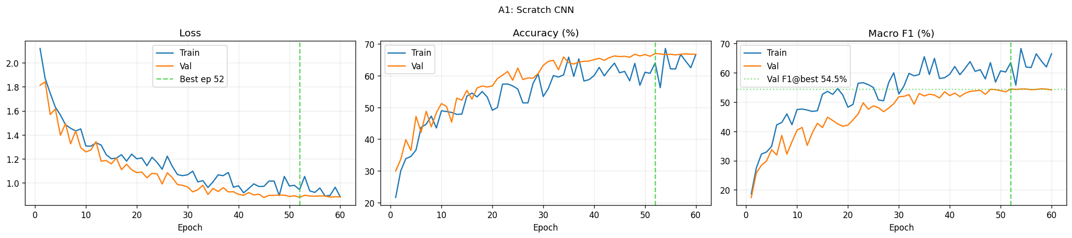
Best checkpoint: epoch 52, held-out macro F1 = 54.49%

5.1.3Results

A1a achieves 66.99% accuracy and macro F1 of 54.49% (Table 3, Figure 4), driven by strong performance on class a (recall = 81.71%) and g (82.64%). Classes h and k collapse to 0% recall; m reaches only 27.52% recall despite substantial training support (Figure 5). Filter norms increase progressively from stage 1 to stage 4, indicating deeper stages develop more specialised representations (Figure 6).

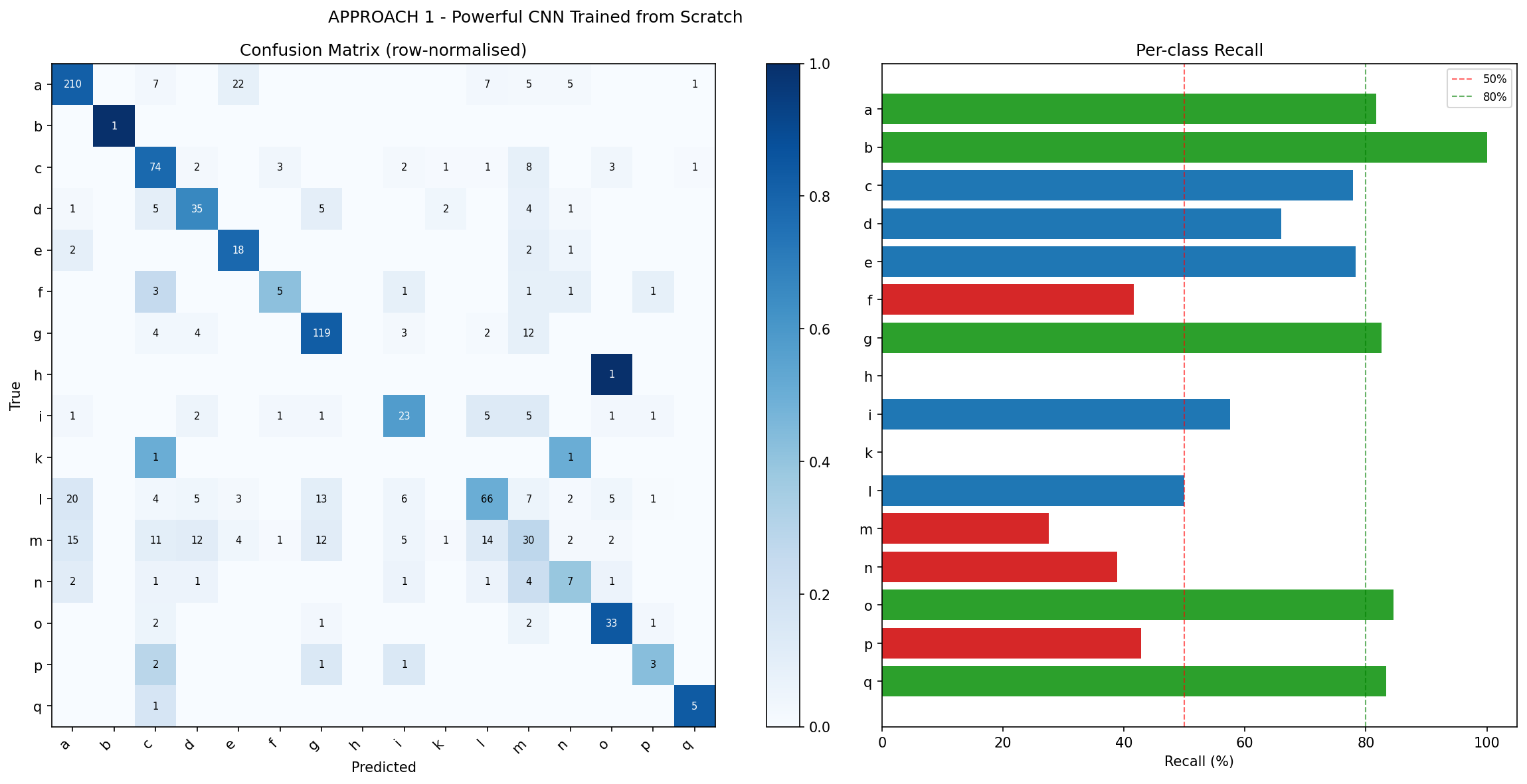
A1a training and validation loss with held-out macro F1 per epoch — Figure 4: A1a training curves: training loss, validation loss, and held-out macro F1 per epoch. The green dashed line marks the best checkpoint.

A1a row-normalised confusion matrix and per-class recall — Figure 5: A1a row-normalised confusion matrix on the held-out test set. Rows are true labels; columns are predicted labels; each cell shows the fraction of true-class samples assigned to each predicted class, so the diagonal represents per-class recall. `m` is largely confused with `n` and `l`.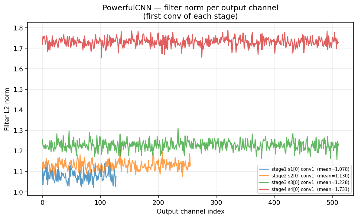

A1a per-channel filter norms by stage — Figure 6: A1a learned filter norms. The plot shows the L2 norm of filters from the first convolutional layer of each stage, illustrating the gradual increase in filter magnitude across deeper network stages.

5.2A1b: SE-ResNet50 from Scratch

5.2.1Architecture

SE-ResNet50 [3] replaces each bottleneck's output with a Squeeze-and-Excitation (SE) block that recalibrates channel responses via global average pooling and a two-layer FC gating network (reduction ratio = 16). The network has 27.08 M parameters. The head replaces the ImageNet classifier with Flatten → Dropout(0.30) → FC(512) → ReLU → Dropout(0.15) → FC(16). The SE bottleneck block is illustrated in Figure 7.

(a) Standard Bottleneck

Conv 1×1BatchNormReLUConv 3×3BatchNormReLUConv 1×1BatchNorm+ReLU

(b) SE-Bottleneck

Conv 1×1BatchNormReLUConv 3×3BatchNormReLUConv 1×1BatchNorm×+ReLU

AvgPool + FC ↓rReLUFC ↑r + Sigmoid

Figure 7: Bottleneck block comparison. (a) Standard ResNet-50 bottleneck. (b) SE-augmented bottleneck [3]: after the final BN the SE branch applies global average pooling, an FC layer that reduces channels by factor r = 16, ReLU, then an FC layer restoring channels followed by Sigmoid, producing a per-channel gate that modulates (×) the bottleneck output before the residual addition (+). Orange = conv, yellow = BN, green = ReLU, cyan = squeeze, purple = excitation; dashed red = skip.

5.2.2Training

Optimizer, scheduler and stopping rule: as A1a (Section 5.1)
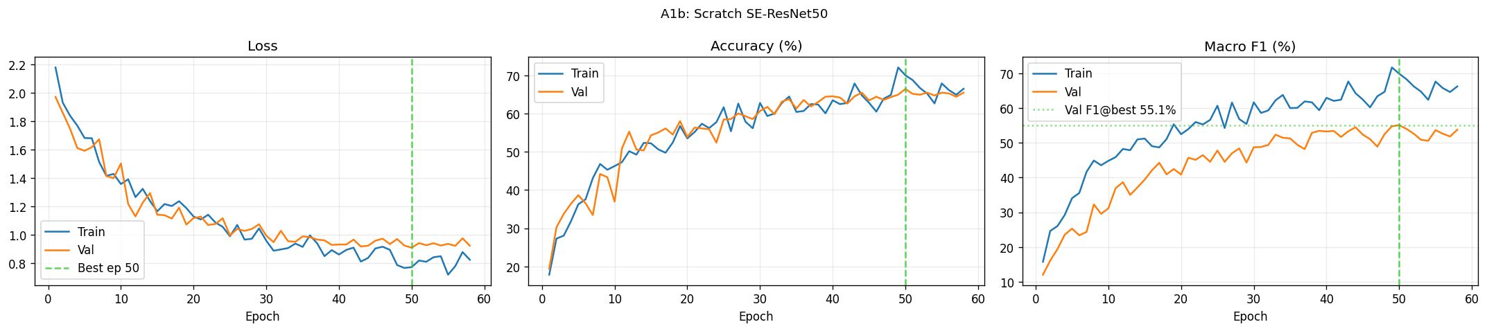
Best checkpoint: epoch 50, held-out macro F1 = 55.07%

5.2.3Results

A1b achieves 66.45% accuracy and macro F1 of 55.07%, closely matching A1a in accuracy (−0.54 pp) while edging it by +0.58 pp macro F1 (Table 3, Figure 8, Figure 9). Layer 4 exhibits the highest mean filter norm, consistent with SE gates concentrating discriminative weight in the final stage (Figure 10).

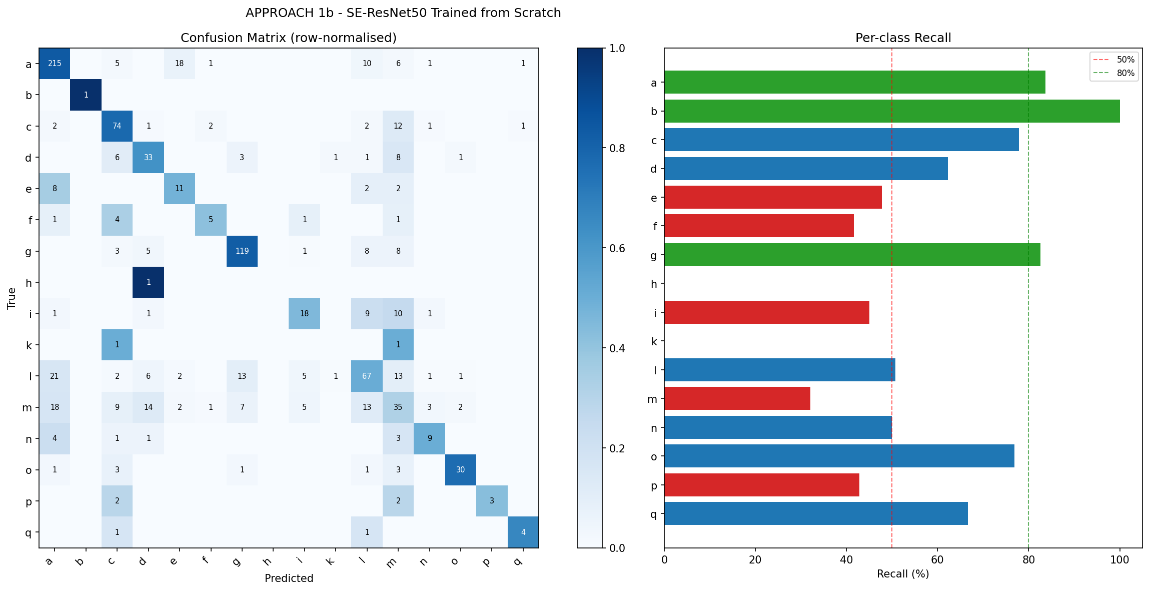
A1b training and validation loss with held-out macro F1 per epoch — Figure 8: A1b training curves: training loss, validation loss, and held-out macro F1 per epoch.

A1b row-normalised confusion matrix and per-class recall — Figure 9: A1b row-normalised confusion matrix on the held-out test set. Classes `h` and `k` collapse to 0% recall; `m` and `i` remain poorly separated.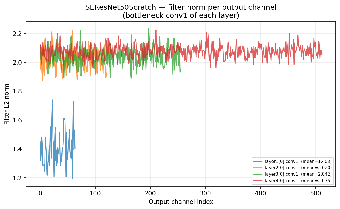

A1b per-channel weight norms by ResNet layer — Figure 10: A1b learned filter norms. Each line shows the L2 norm per output channel for the bottleneck Conv1×1 of each ResNet layer; layer 4 (512→2048) has the highest mean norm (∼0.23).

6Approach 2 — Fine-Tuned Pretrained Backbones

6.1A2a: ConvNeXt-Small Fine-Tuned

6.1.1Architecture and Transfer-Learning Strategy

ConvNeXt-Small [8] (49.86 M total parameters) is fine-tuned on the petri dish domain. Stages 0–1 (stem and first downsampling stage, 0.24 M parameters) are frozen; the remaining 49.61 M parameters receive discriminative learning rates:

η6 × 10⁻⁶features[2] (early backbone)1.8 × 10⁻⁵features[3–5] (mid backbone)6 × 10⁻⁵features[6–7] (late backbone)3 × 10⁻⁴GeM pool + head

(3)

The original adaptive average pooling is replaced by learnable GeM pooling (Section 5.1), and the ImageNet head is replaced by: Flatten → LayerNorm(768) → Dropout(0.30) → FC(512) → GELU → Dropout(0.15) → FC(16). The layer-group learning-rate scheme is depicted in Figure 11.

Features[0–1]
frozenη = 0Features[2]6×10⁻⁶Features[3–5]1.8×10⁻⁵Features[6–7]6×10⁻⁵GeM Pool
+ Head3×10⁻⁴

Figure 11: ConvNeXt-Small layer-group fine-tuning strategy. Features[0–1] (stem and first downsampling stage, 0.24 M parameters) are frozen (grey). Remaining groups receive progressively higher learning rates (orange → green) as depth increases, from 6×10⁻⁶ for the earliest unfrozen group up to 3×10⁻⁴ for the GeM pool and classification head (Eq. 3).

6.1.2Training

Optimizer: AdamW, weight decay = 2×10⁻⁴
Scheduler: Linear warm-up (5 epochs) then CosineAnnealingLR (T_max = 35, η_min = 10⁻⁷)
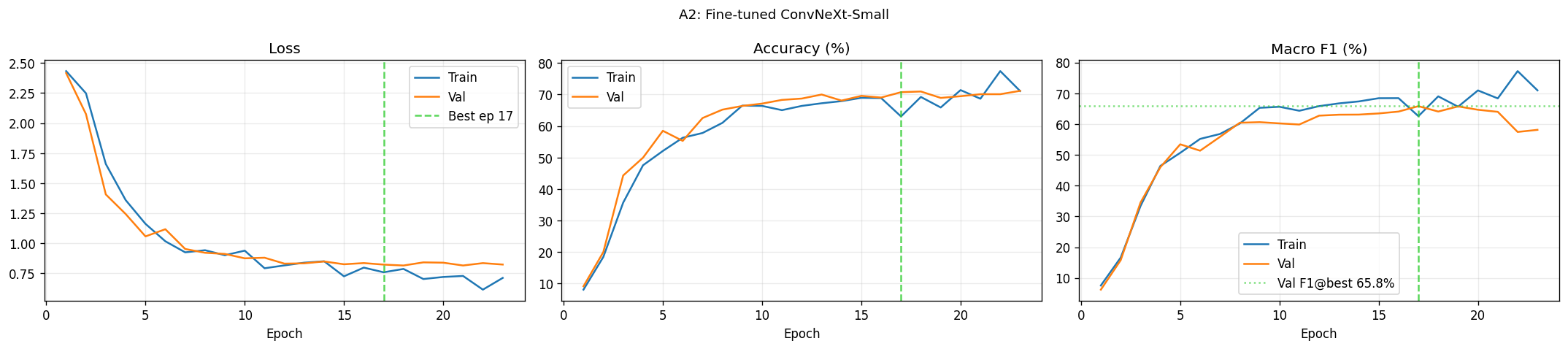
Max epochs: 40; patience: 6; best checkpoint: epoch 17, macro F1 = 65.81%

6.1.3Results

A2a achieves the best accuracy (70.71%) and best macro F1 (65.81%) among all six approaches (Table 3, Figure 12, Figure 13). ImageNet pretraining yields +3.72 pp accuracy and +11.32 pp macro F1 over A1a. Higher filter norms relative to scratch CNNs confirm that ImageNet-initialised weights retain strong feature magnitudes after domain adaptation (Figure 14).

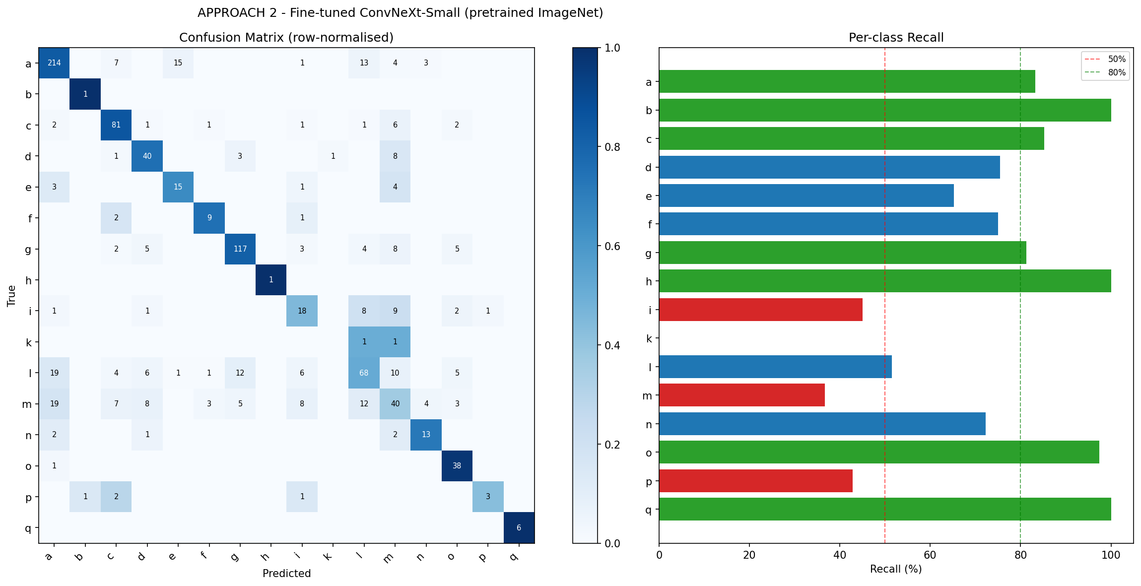
A2a training and validation loss with held-out macro F1 per epoch — Figure 12: A2a (ConvNeXt-Small fine-tuned) training curves: training loss, validation loss, and held-out macro F1 per epoch. Early stopping triggers at epoch 23 (patience = 6); convergence is substantially faster than for the scratch CNNs.

A2a row-normalised confusion matrix and per-class recall — Figure 13: A2a (ConvNeXt-Small fine-tuned) row-normalised confusion matrix on the held-out test set. Class `k` remains at 0% recall and `m` at 36.70%; both overlap with morphologically similar classes.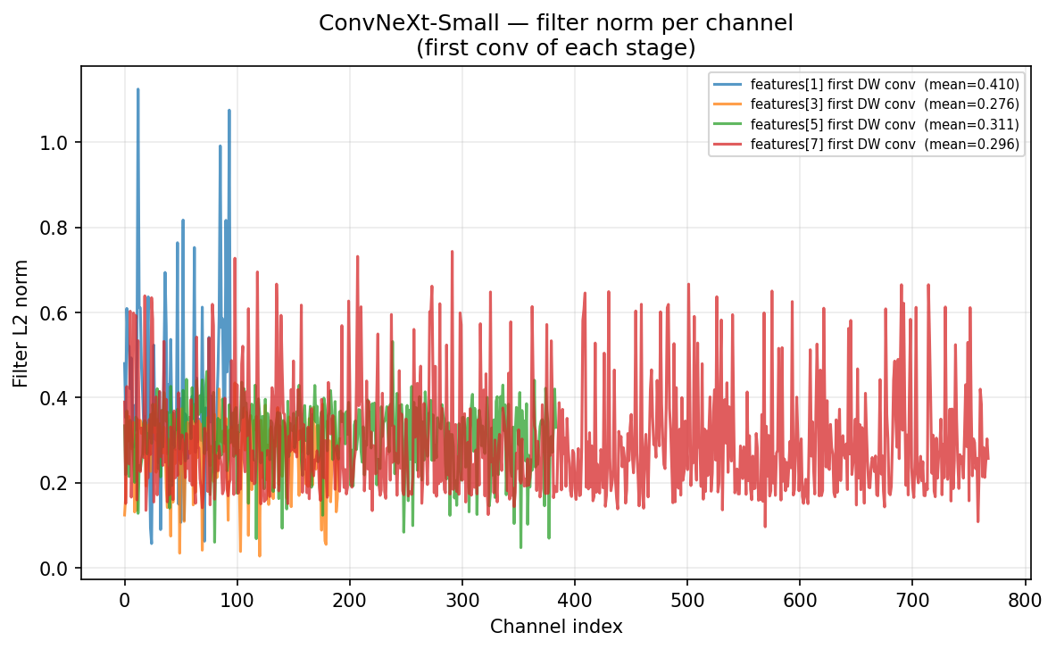

A2a per-channel depthwise convolution norms by stage — Figure 14: A2a (ConvNeXt-Small fine-tuned) learned filter norms. Each line shows the per-channel L2 norm of the first depthwise convolution in each ConvNeXt stage after fine-tuning; compare the scratch CNN in Figure 6.

6.2A2b: Swin-T Fine-Tuned

6.2.1Architecture and Transfer-Learning Strategy

Swin Transformer (Tiny) [7] (27.92 M total parameters) uses hierarchical windowed self-attention with shifted windows, producing a 768-d representation. Features 0–2 (patch embedding, Stage 1, first downsampling, 0.30 M parameters) are frozen; features 3–7, the layer norm, and the custom head receive discriminative rates:

η3 × 10⁻⁶features[3] (newly unfrozen stage 2)1.8 × 10⁻⁵features[4–5] (stages 3–4)6 × 10⁻⁵features[6–7] + LayerNorm3 × 10⁻⁴custom head

(4)

The original classification head is replaced by: LayerNorm(768) → Dropout(0.30) → FC(512) → GELU → Dropout(0.15) → FC(16). The layer-group learning-rate scheme is depicted in Figure 15.

Features[0–2]
frozenη = 0Features[3]3×10⁻⁶Features[4–5]1.8×10⁻⁵Features[6–7]
+ LayerNorm6×10⁻⁵Custom
Head3×10⁻⁴

Figure 15: Swin-T layer-group fine-tuning strategy. Features[0–2] (patch embedding, Stage 1, and first downsampling block, 0.30 M parameters) are frozen (grey). Remaining groups receive progressively higher learning rates (orange → green), from 3×10⁻⁶ for the newly unfrozen Stage 2 up to 3×10⁻⁴ for the classification head (Eq. 4).

6.2.2Training

Optimizer, scheduler and stopping rule: as A2a (Section 6.1)
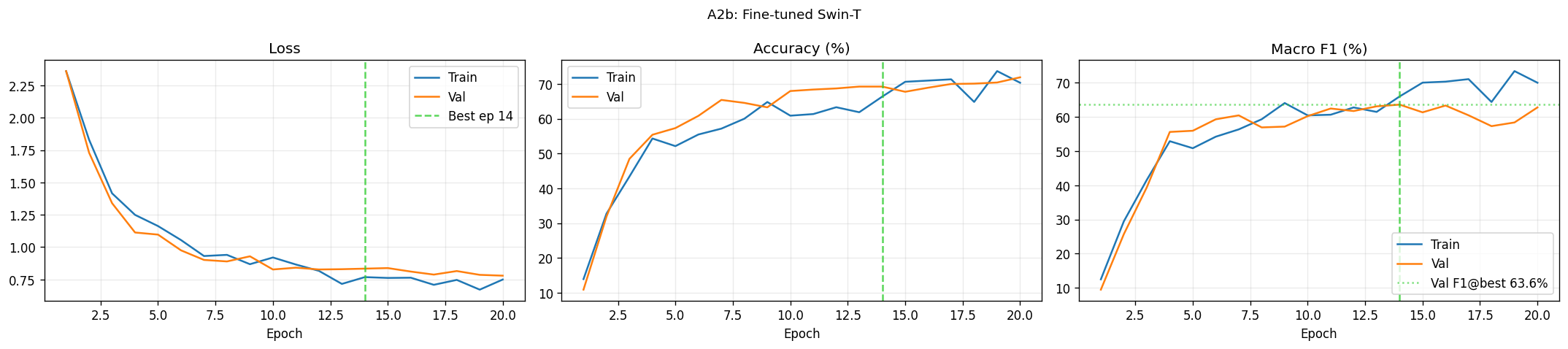
Best checkpoint: epoch 14, held-out macro F1 = 63.59%

6.2.3Results

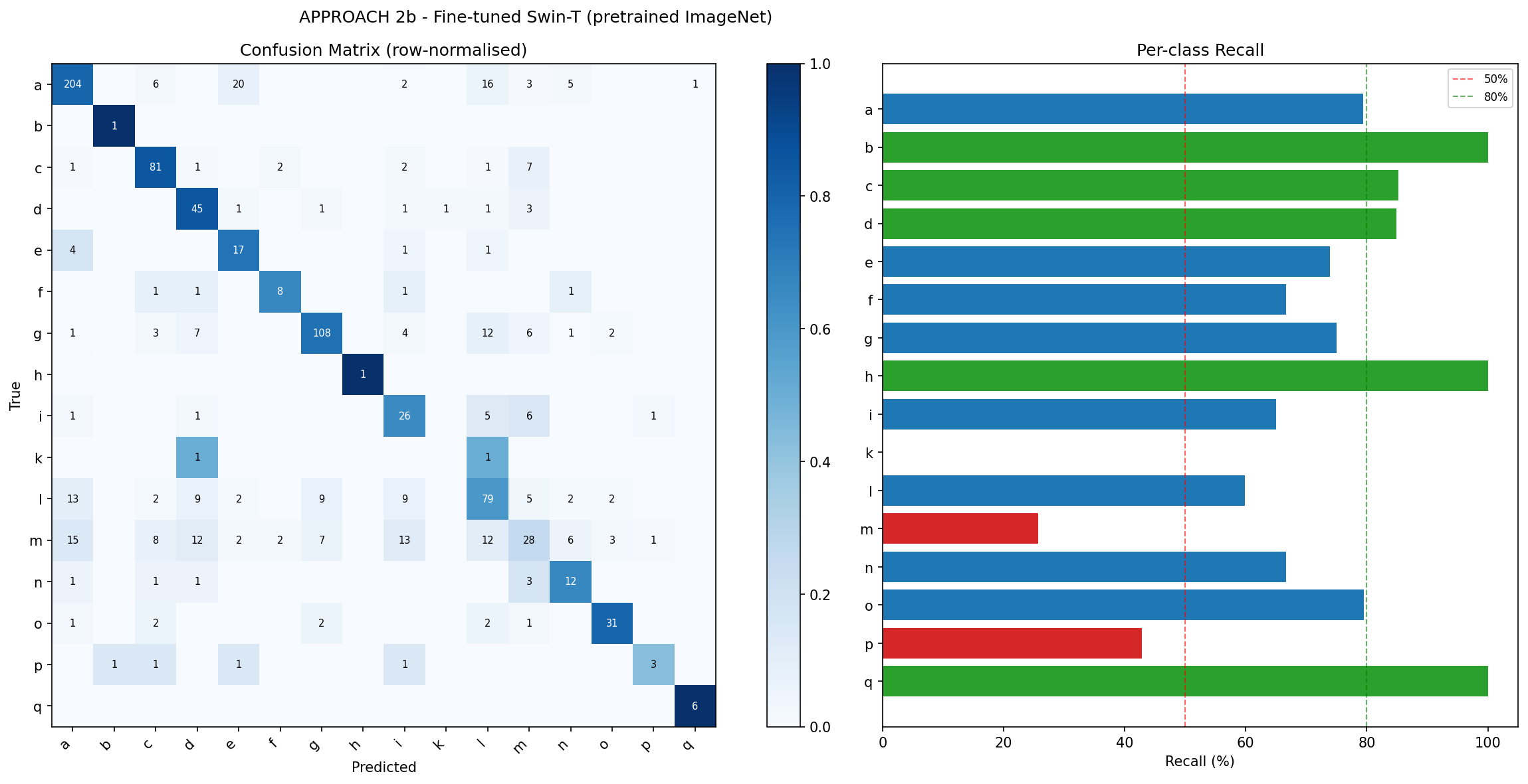
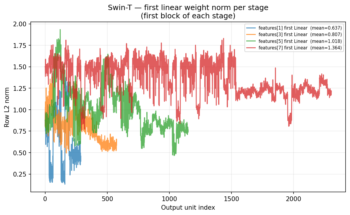
A2b achieves 69.22% accuracy and 63.59% macro F1, trailing A2a by 1.49 pp accuracy and 2.22 pp macro F1 (Table 3, Figure 16, Figure 17). Class k (0% recall) is the sole persistent failure. A2b does retain a 7 pp F1 advantage over A2a on class i, while A2a excels on n (+15 pp) and m (+7 pp). The sharp norm increase at features[7] shows the deepest unfrozen stage specialises most strongly after fine-tuning (Figure 18).

A2b training and validation loss with held-out macro F1 per epoch — Figure 16: A2b (Swin-T fine-tuned) training curves: training loss, validation loss, and held-out macro F1 per epoch. Early stopping triggers at epoch 20.

A2b row-normalised confusion matrix and per-class recall — Figure 17: A2b (Swin-T fine-tuned) row-normalised confusion matrix on the held-out test set.

A2b per-row query/key/value projection norms by stage — Figure 18: A2b (Swin-T fine-tuned) learned weight norms. Each line shows the per-row L2 norm of the first linear projection (query/key/value) in each Swin-T stage after fine-tuning.

7Approach 3 — Pretrained Embeddings + RBF-SVM

The fine-tuned backbones are used as frozen feature extractors; their 768-d representations are standardised (StandardScaler [10]) and classified with a balanced RBF-SVM [13] (class_weight="balanced"). Hyperparameters C and γ are selected by 3-fold cross-validation over C ∈ {0.1, 0.5, 1, 5, 10} and γ ∈ {scale, 5×10⁻⁴, 10⁻³}, optimising macro F1. The procedure is given in Listing 4.

Listing 4: Approach 3: pooled 768-d embeddings from a frozen fine-tuned backbone, standardised and classified by a balanced RBF-SVM whose C and γ are chosen by 3-fold grid search on macro F1.

@torch.no_grad()
def embed(backbone: nn.Module, loader: DataLoader) -> np.ndarray:
    # The fine-tuned backbone, frozen, up to its pooled 768-d features.
    backbone.eval()
    return np.concatenate([backbone(x).cpu().numpy() for x, _ in loader])

Z_train, Z_test = embed(backbone, train_loader), embed(backbone, test_loader)

svm = make_pipeline(StandardScaler(),
                    SVC(kernel="rbf", class_weight="balanced"))
grid = GridSearchCV(svm,
                    {"svc__C": [0.1, 0.5, 1, 5, 10],
                     "svc__gamma": ["scale", 5e-4, 1e-3]},
                    cv=3, scoring="f1_macro")
grid.fit(Z_train, y_train)      # refits the best (C, gamma) on all of Z_train
y_pred = grid.predict(Z_test)

7.1A3a: ConvNeXt-Small Embeddings + SVM

Image320²×3ConvNeXt-Small
backbone (frozen)feature mapsGeM Pool768-dStandard
Scalerμ = 0, σ = 1RBF-SVM
C = 52603 SVsClass

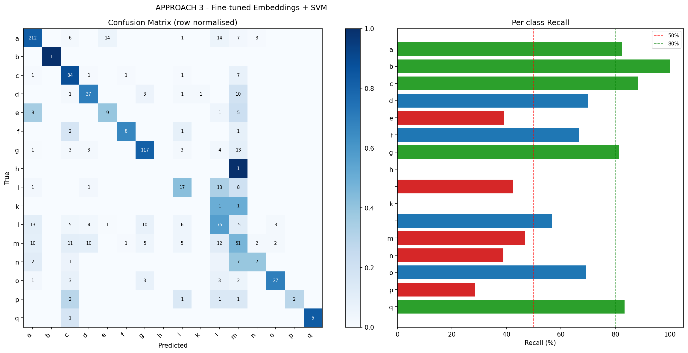
Figure 19: A3a inference pipeline. The ConvNeXt-Small backbone is frozen at the A2a fine-tuned weights; GeM pooling yields a 768-d embedding that is standardised before RBF-SVM classification.

Grid-search CV yields macro F1 = 0.8723 (see Figure 19 for hyperparameters). Results in Table 3 and Figure 20.

The CV score sits far above the 58.01% held-out macro F1 because the folds are drawn from the same training images the backbone was fine-tuned on: their embeddings are more separable than those of images the backbone has never seen. It is used only to rank hyperparameters, not as an estimate of test performance.

A3a row-normalised confusion matrix and per-class recall — Figure 20: A3a (ConvNeXt-Small+SVM) row-normalised confusion matrix on the held-out test set.

7.2A3b: Swin-T Embeddings + SVM

Best hyperparameters: C = 10, γ = 5×10⁻⁴, 2 431 support vectors (CV macro F1 = 0.8630). Results in Table 3 and Figure 21.

A3b row-normalised confusion matrix and per-class recall — Figure 21: A3b (Swin-T+SVM) row-normalised confusion matrix on the held-out test set.

8Comparative Analysis

8.1Overall Performance

Table 3: Full held-out test comparison. Best value per metric in bold.

Metric	A1a	A1b	A2a	A2b	A3a	A3b
	Scratch CNN	Scratch SE-R50	ConvNeXt FT	Swin-T FT	ConvNeXt+SVM	Swin-T+SVM
Accuracy	66.99%	66.45%	70.71%	69.22%	69.44%	70.61%
Macro Prec.	53.38%	58.43%	64.51%	61.36%	63.35%	64.05%
Macro Recall	57.06%	53.77%	69.45%	69.04%	55.87%	55.78%
Macro F1	54.49%	55.07%	65.81%	63.59%	58.01%	58.57%
Weighted F1	66.46%	66.16%	70.14%	68.83%	69.46%	70.47%

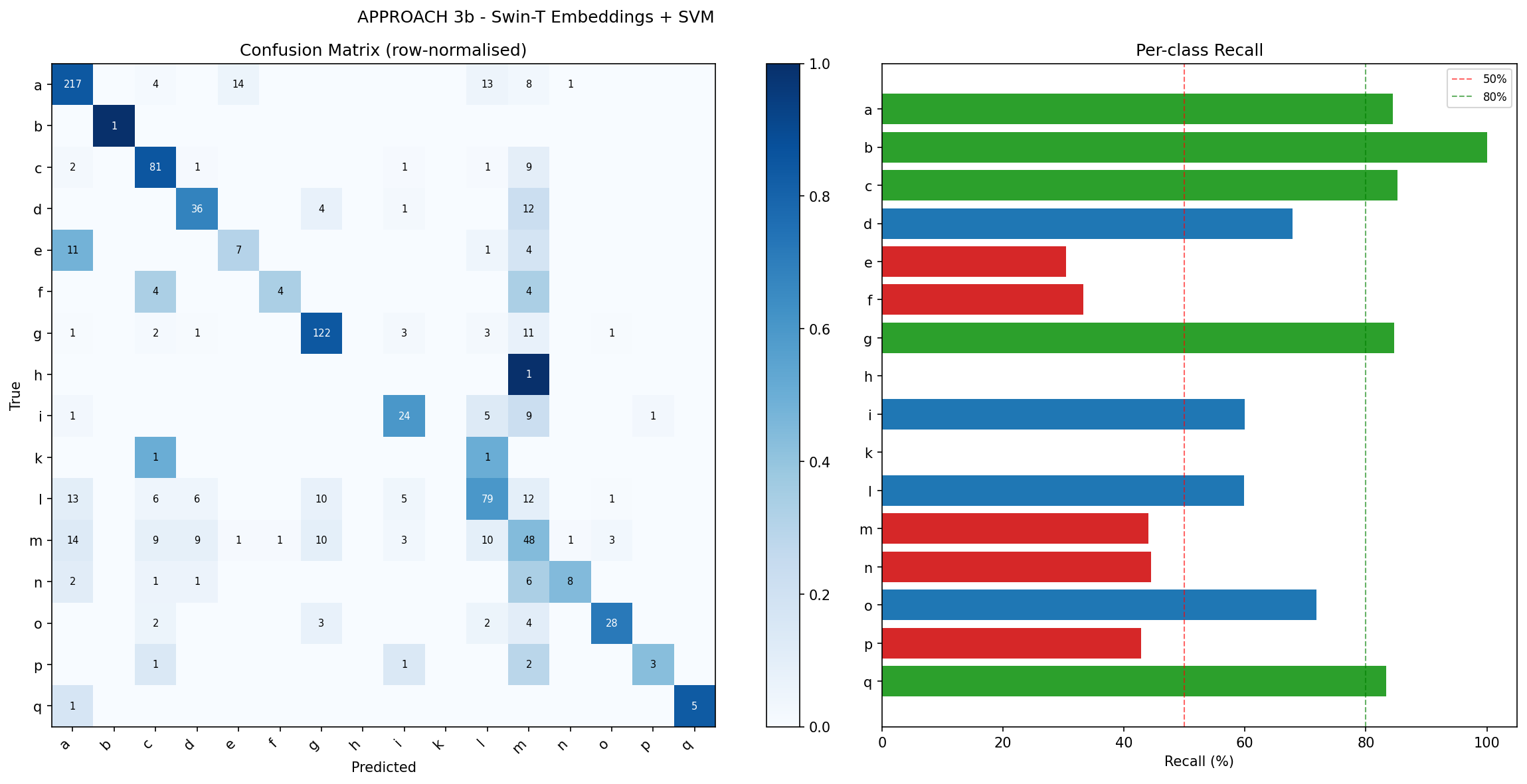
A2a leads on accuracy (70.71%), macro precision, macro recall, and macro F1 (65.81%). A3b achieves the highest weighted F1 (70.47%) but trails A2a by 7.24 pp macro F1. Both pretrained backbones substantially outperform scratch CNNs; the SVM approaches match or exceed fine-tuned accuracy but trail by 7–8 pp macro F1.

8.2Per-Class Analysis

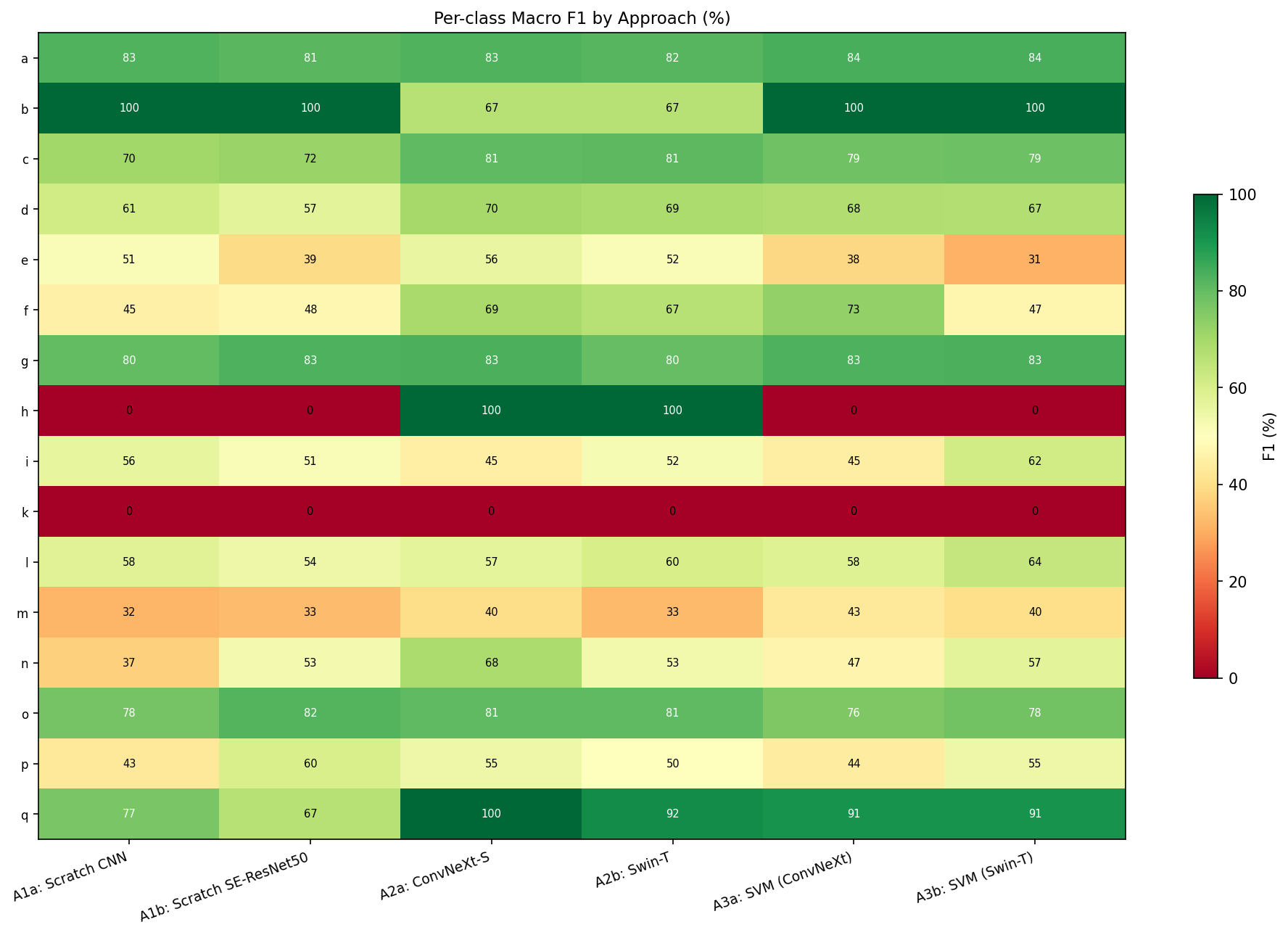
Several patterns emerge from Figure 22:

Consistently easy (a, b, g, o): high F1 across all approaches. Large sample count (a, g) or visually distinctive morphology (b, o).
Consistently hard (k, m, i): ≤ 52% F1 for all approaches. t-SNE (Figure 23) confirms that their embeddings overlap with neighbouring classes.
Class h (5 training samples): 100% recall under A2a and A2b, 0% under every other approach (see Section 9).
A2a over A2b for n (+15.1 pp F1), m (+7.1 pp), and q (+7.7 pp): ConvNeXt's depthwise convolutions better capture the texture patterns distinguishing these classes. A2b retains an advantage on class i (+7.0 pp).

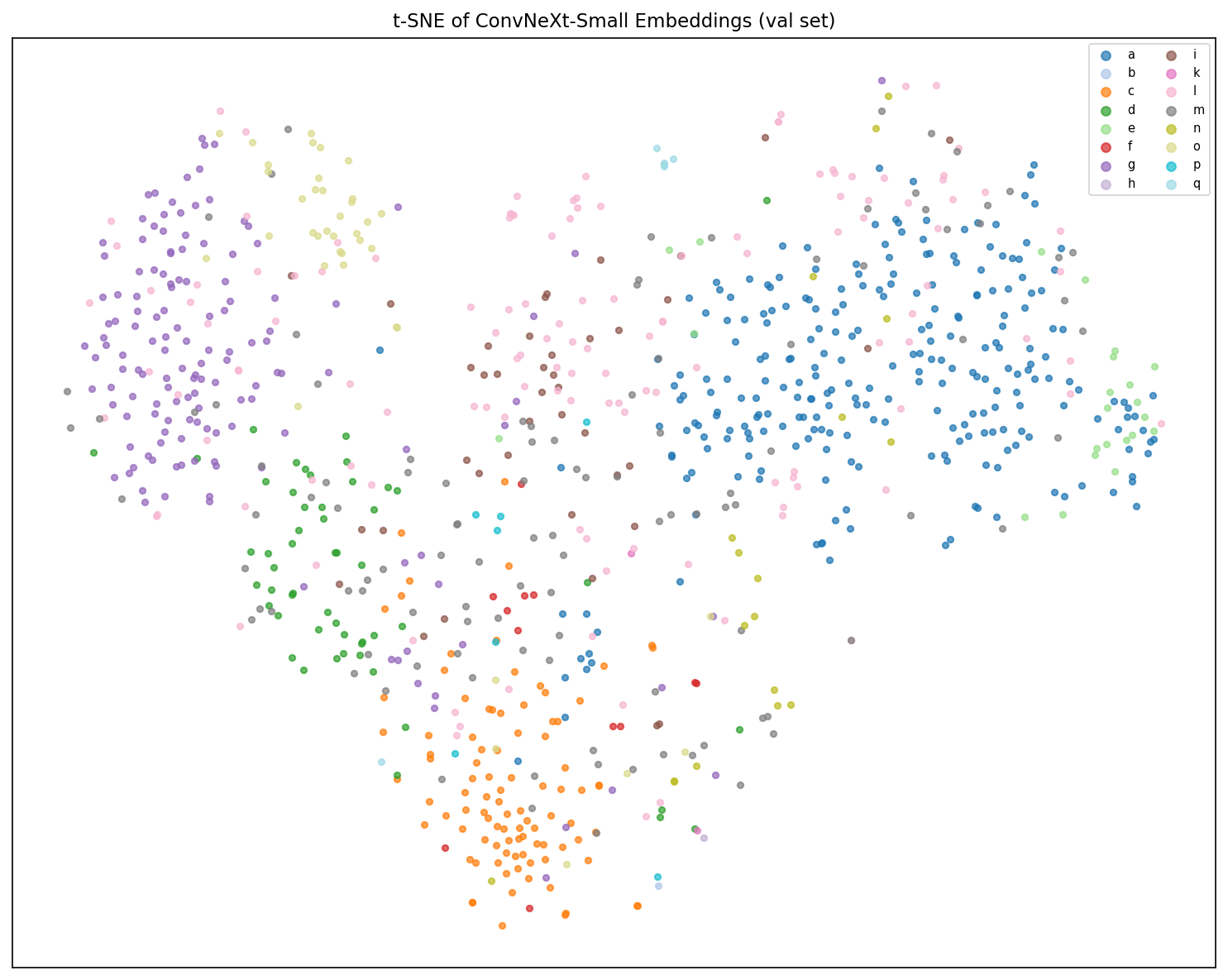
Heatmap of per-class macro F1 for all six approaches — Figure 22: Per-class F1 for all six approaches. Darker cells indicate higher F1.

Two-dimensional t-SNE projection of ConvNeXt-Small embeddings — Figure 23: 2-D t-SNE [14] projection of ConvNeXt-Small embeddings on the validation set. Each point represents one sample, coloured by ground-truth class label. Most classes form tight, well-separated clusters, consistent with A2a's high accuracy. Classes `d`/`i` and `l`/`m` form intermixed regions, explaining their persistently low recall across all approaches.

9Discussion

Why SVM classifiers underperform their backbone fine-tuned models on macro F1. A3a trails A2a by 7.8 pp macro F1; A3b trails A2b by 5.0 pp, despite using embeddings from the same frozen backbones. Two effects compound: (1) the SVM's margin objective prioritises precision over recall on rare classes (f: 80% precision but 33–67% recall in A3a/A3b); (2) the balanced class-weight flag cannot recover rare classes (h, k) whose frozen embeddings overlap majority-class clusters.

Why fine-tuned backbones dominate scratch CNNs on ultra-rare classes. Class h (5 training samples) achieves 100% recall under A2a/A2b but 0% under all scratch and SVM approaches. The ImageNet prior encodes low-level visual structure that generalises immediately from a single example; scratch CNNs lack this prior and collapse the class into a majority-class cluster, an effect that neither data augmentation nor WeightedRandomSampler can overcome with only 5 training samples.

10Conclusion

Six approaches were evaluated on the same 939-sample held-out test set. Fine-tuned ConvNeXt-Small (A2a) is the pick, with the best accuracy (70.71%) and macro F1 (65.81%). The embedding + SVM variants match its accuracy but give up 7–8 pp of macro F1 on the rare classes, and the scratch CNNs trail on both.

References

[1]Antoni Buades, Bartomeu Coll, and J-M Morel. A non-local algorithm for image denoising. In 2005 IEEE computer society conference on computer vision and pattern recognition (CVPR'05), volume 2, pages 60–65. Ieee, 2005.
[2]Kaiming He, Xiangyu Zhang, Shaoqing Ren, and Jian Sun. Identity mappings in deep residual networks. In European conference on computer vision, pages 630–645. Springer, 2016.
[3]Jie Hu, Li Shen, and Gang Sun. Squeeze-and-excitation networks. In Proceedings of the IEEE conference on computer vision and pattern recognition, pages 7132–7141, 2018.
[4]Gao Huang, Yu Sun, Zhuang Liu, Daniel Sedra, and Kilian Q Weinberger. Deep networks with stochastic depth. In European conference on computer vision, pages 646–661. Springer, 2016.
[5]Glenn Jocher, Ayush Chaurasia, and Jing Qiu. Ultralytics YOLOv8, 2023. Version 8.0.0, https://github.com/ultralytics/ultralytics.
[6]Tsung-Yi Lin, Priya Goyal, Ross Girshick, Kaiming He, and Piotr Dollár. Focal loss for dense object detection. In Proceedings of the IEEE international conference on computer vision, pages 2980–2988, 2017.
[7]Ze Liu, Yutong Lin, Yue Cao, Han Hu, Yixuan Wei, Zheng Zhang, Stephen Lin, and Baining Guo. Swin transformer: Hierarchical vision transformer using shifted windows. In Proceedings of the IEEE/CVF international conference on computer vision, pages 10012–10022, 2021.
[8]Zhuang Liu, Hanzi Mao, Chao-Yuan Wu, Christoph Feichtenhofer, Trevor Darrell, and Saining Xie. A convnet for the 2020s. In Proceedings of the IEEE/CVF conference on computer vision and pattern recognition, pages 11976–11986, 2022.
[9]Ilya Loshchilov and Frank Hutter. Decoupled weight decay regularization. arXiv preprint arXiv:1711.05101, 2017.
[10]Fabian Pedregosa, Gaël Varoquaux, Alexandre Gramfort, Vincent Michel, Bertrand Thirion, Olivier Grisel, Mathieu Blondel, Peter Prettenhofer, Ron Weiss, Vincent Dubourg, et al. Scikit-learn: Machine learning in Python. Journal of machine learning research, 12:2825–2830, 2011.
[11]Filip Radenović, Giorgos Tolias, and Ondřej Chum. Fine-tuning cnn image retrieval with no human annotation. IEEE transactions on pattern analysis and machine intelligence, 41(7):1655–1668, 2018.
[12]Ali M Reza. Realization of the contrast limited adaptive histogram equalization (clahe) for real-time image enhancement. Journal of VLSI signal processing systems for signal, image and video technology, 38(1):35–44, 2004.
[13]Ali Sharif Razavian, Hossein Azizpour, Josephine Sullivan, and Stefan Carlsson. Cnn features off-the-shelf: an astounding baseline for recognition. In Proceedings of the IEEE conference on computer vision and pattern recognition workshops, pages 806–813, 2014.
[14]Laurens Van der Maaten and Geoffrey Hinton. Visualizing data using t-sne. Journal of machine learning research, 9(11), 2008.
[15]Sanghyun Woo, Jongchan Park, Joon-Young Lee, and In So Kweon. Cbam: Convolutional block attention module. In Proceedings of the European conference on computer vision (ECCV), pages 3–19, 2018.

Contents