Acoustic Species Identification in the Pantanal
Ting Tang
19 June 2026
Contents
- 1Task
- 2Dataset
- 3Related Work
- Pretrained bioacoustic encoders.
- Image backbones for audio.
- Class imbalance and regularisation.
- Generative data augmentation.
- 4Audio Feature Extraction
- 4.1BirdNET Embeddings
- 4.2Log-Mel Spectrograms
- 5Experiment A — Models on Original Data
- 5.1A1: BirdNET Embeddings + Classical ML
- 5.2A1 MLP Architecture
- 5.3A2: Fine-tuned Heads and Backbones
- BirdNET replacement heads.
- Spectrogram backbone + embedding fusion.
- 5.4From-Scratch Spectrogram CNNs
- 6Experiment B — AudioLDM2 Data Augmentation
- 6.1AudioLDM2 Synthesis Pipeline
- 6.2Synthetic Sample Generation
- 6.3Retraining on the Augmented Data
- 7Results
- 7.1Macro ROC-AUC Summary
- 7.2Per-Class Analysis
- 8Discussion
- Choosing a from-scratch model.
- Effect of AudioLDM2 augmentation.
- Singleton recovery.
- Limitations.
- 9Conclusion
1Task
The BirdCLEF 2026 challenge [1] predicts species presence in audio from the Brazilian Pantanal. The train_audio recordings are split 80 / 20 into train and validation, and two experiments are run:
- Experiment A — models trained on the original, imbalanced data.
- Experiment B — the same models retrained after balancing the rare classes with synthetic audio from AudioLDM2 [2].
Three approaches are benchmarked: BirdNET embeddings with ML classifiers, BirdNET fine-tuning, and a model trained from scratch.
- A1/B1 — embeddings + classical ML. BirdNET embeddings with LightGBM, logistic regression and an MLP.
- A2/B2 — fine-tuning. Two BirdNET heads on the frozen embeddings (linear and one-hidden-layer), plus two pretrained spectrogram backbones (AST-style ViT-Base and ConvNeXt-Small) fine-tuned and fused with the embedding.
- From scratch. Two randomly initialized spectrogram CNNs (EfficientNet-B2 and PANNs CNN14) trained on log-mel spectrograms with no BirdNET signal.
All models are scored by macro-averaged ROC-AUC on the held-out validation set, which weights every species equally on this long-tailed corpus.
2Dataset
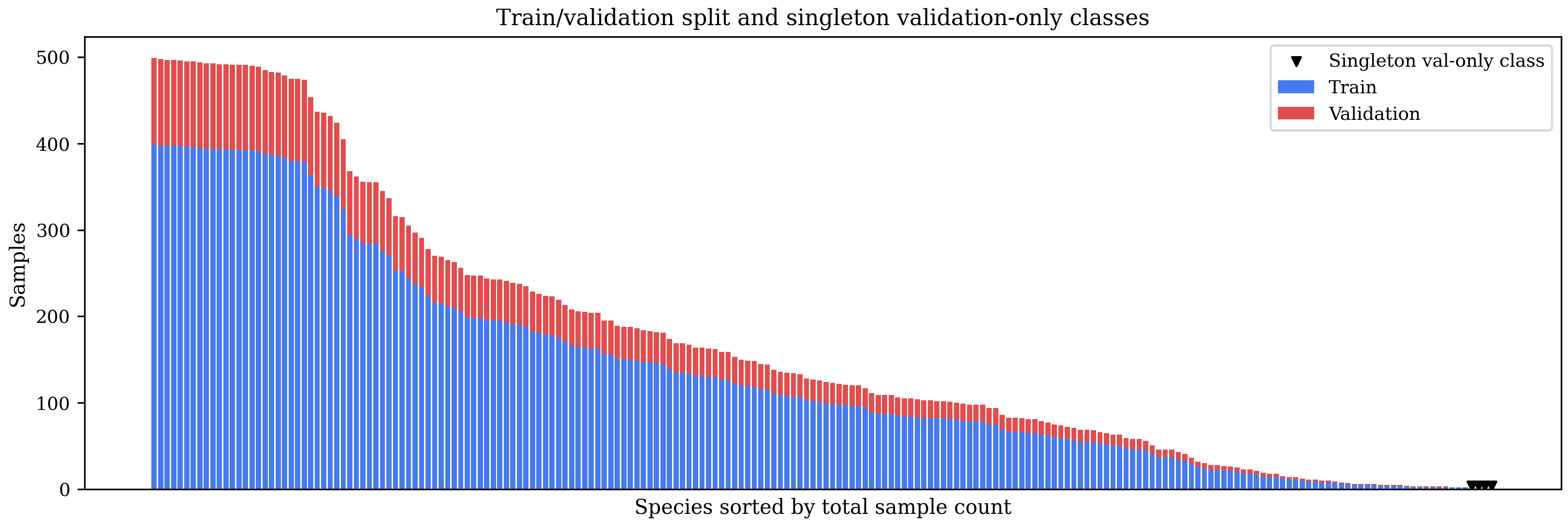
The corpus has 35,549 recordings covering 206 species, resampled to 48 kHz and split 80 / 20 by stratified sampling on primary_label. Singleton classes cannot be stratified, so they are placed in validation.
| Split | Files | Classes | Singletons |
|---|---|---|---|
| Train | 28,436 | 202 | 0 |
| Validation | 7,113 | 206 | 4 |
3Related Work
Pretrained bioacoustic encoders.BirdNET [3] is the standard transfer-learning backbone for bird sound recognition, trained on millions of labelled recordings and the reference baseline across recent BirdCLEF editions [4]. Its penultimate 1024-d activation is a general-purpose acoustic embedding, reused here both as a fixed feature extractor (route A1 and the BirdNET fine-tune heads) and as a fusion signal alongside spectrogram backbones. After L2 normalisation e = e/‖e‖2, cosine similarity reduces to a dot product
removing magnitude bias so every downstream classifier operates on a common scale.
Image backbones for audio.Treating a spectrogram as an image lets ImageNet-pretrained vision models transfer to audio. The Audio Spectrogram Transformer [5] applies a ViT directly to spectrogram patches, while ConvNeXt [6] modernises the ConvNet design; both are fine-tuned here. As BirdNET-free baselines, EfficientNet-B2 [7] and the audio-native PANNs CNN14 [8] are trained from random initialisation, isolating how much performance is attributable to BirdNET's pretraining.
Class imbalance and regularisation.Long-tailed audio datasets motivate loss- and sampling-level corrections. Focal loss [9] down-weights easy examples, concentrating gradient mass on rare species:
where pt is the model probability for the true class, αt an inverse-frequency class weight, and γ ≥ 0 a focusing parameter (γ = 0 recovers weighted cross-entropy). Mixup [10] regularises by training on convex combinations
softening decision boundaries where acoustically similar species overlap. SpecAugment [11] masks contiguous time and frequency bands to discourage over-fitting. All three are used in the fine-tuning and from-scratch routes.
Generative data augmentation.Rather than perturbing existing clips, AudioLDM2 [2] synthesises new audio from a text prompt via latent diffusion. Experiment B uses the pretrained model to manufacture training clips for under-represented and singleton species — novel signal that conventional augmentation cannot provide.
4Audio Feature Extraction
4.1BirdNET Embeddings
Embeddings come from BirdNET v2.4 [3, 4]. Each file is loaded at 48 kHz mono, split into non-overlapping 3-second chunks, and passed through BirdNET for one 1024-d vector per chunk; one chunk per training file is retained for tractable runtime. Vectors are then L2-normalised as in Section 3 (Listing 1).
def get_embeddings(chunks: list[np.ndarray]) -> np.ndarray:
    # One 1024-d BirdNET embedding per 3-second mono 48 kHz chunk.
    prepared = [np.pad(y, (0, CHUNK_SAMPLES - len(y)))[:CHUNK_SAMPLES]
                for y in chunks]
    inputs = [(chunk, SR) for chunk in prepared]
    result = _birdnet_model.encode_arrays(inputs, device="CPU", ...)
    return result.embeddings[:, 0, :].astype(np.float32)  # (N, 1024)

def l2_normalize(X: np.ndarray) -> np.ndarray:
    # Unit-normalise rows so cosine distance governs classification.
    norms = np.linalg.norm(X, axis=1, keepdims=True)
    return X / np.maximum(norms, 1e-8)
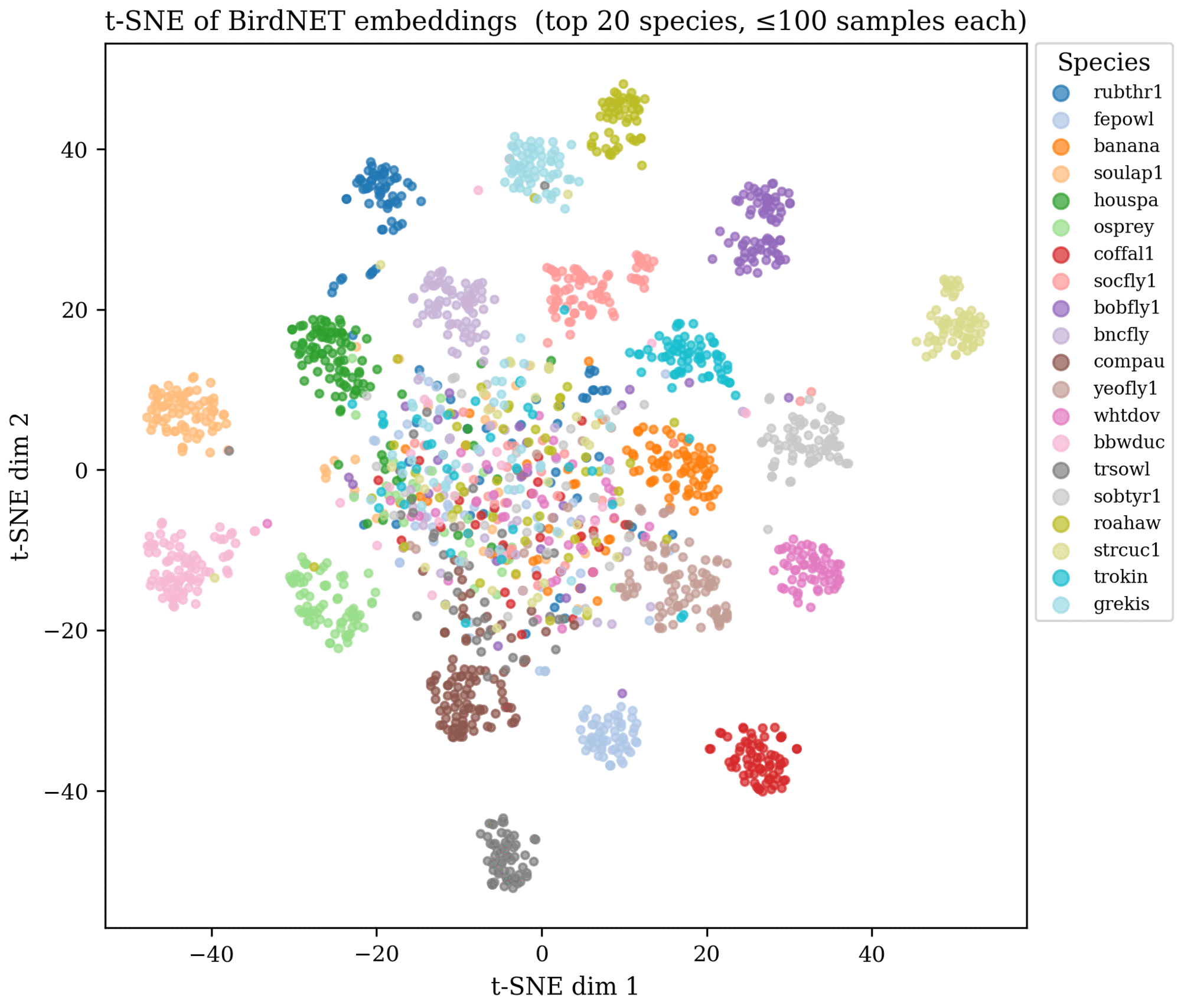
The t-SNE projection of the 20 most populated species (Figure 2) shows mostly compact, well-separated clusters — explaining the high macro-AUC of even a linear classifier — with a crowded centre of acoustically ambiguous classes.
4.2Log-Mel Spectrograms
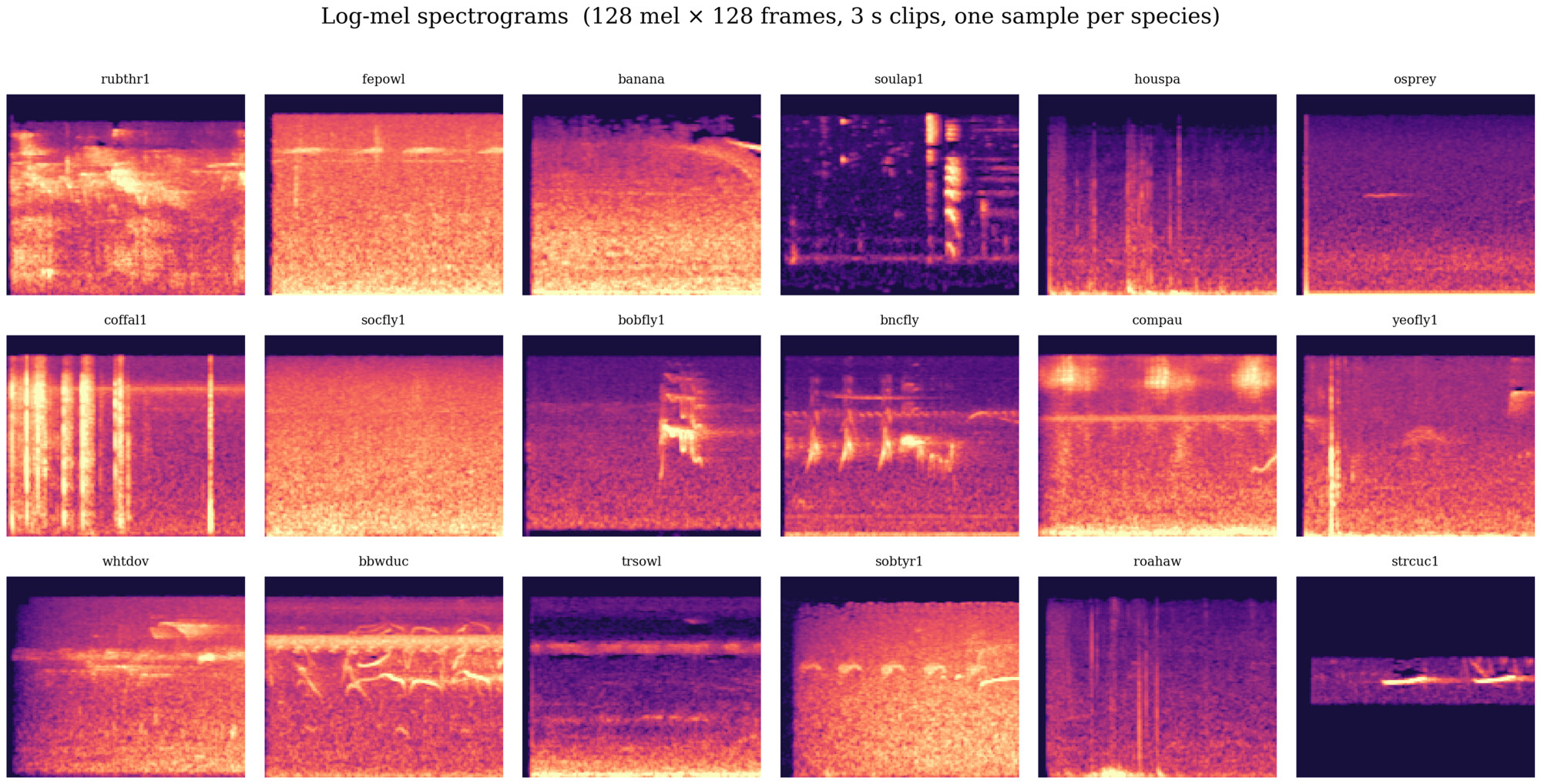
The fine-tuned backbones and from-scratch CNNs instead convert each 3-second clip to a 128 × 128 log-mel spectrogram:
- 128 Mel bands, FFT size 2048, power spectrogram converted to dB with
power_to_db; - time axis zero-padded or truncated to exactly 128 frames;
- the fusion backbones use per-sample min–max scaling to [0, 1]; the from-scratch CNNs use a global mean/standard-deviation normaliser estimated from 500 randomly sampled training clips.
The single-channel image is then resized to each backbone's native resolution — 224 × 224 for the AST/ViT and ConvNeXt fusion models, 260 × 260 for EfficientNet-B2 — while CNN14 consumes the 128 × 128 image directly (Listing 2).
def audio_to_logmel(y, n_mels=128, n_frames=128) -> np.ndarray:
    # 128x128 per-sample-normalised log-mel spectrogram for a 3 s chunk.
    y = np.pad(y, (0, CHUNK_SAMPLES - len(y)))[:CHUNK_SAMPLES]
    hop = CHUNK_SAMPLES // n_frames
    mel = librosa.feature.melspectrogram(
        y=y, sr=SR, n_fft=2048, hop_length=hop,
        n_mels=n_mels, fmin=50, fmax=SR // 2)
    logmel = librosa.power_to_db(mel, ref=np.max)        # to decibels
    logmel = logmel[:, :n_frames]                        # fix time axis
    lo, hi = float(logmel.min()), float(logmel.max())
    return ((logmel - lo) / (hi - lo + 1e-6)).astype(np.float32)
SpecAugment [11] is applied on-the-fly during from-scratch training: a random time mask (up to 30 frames) and frequency mask (up to 15 bins) are zeroed per sample to discourage over-fitting (Listing 3).
def _spec_augment_tensor(mel, max_t=30, max_f=15):
    mel = mel.clone()
    _, f_dim, t_dim = mel.shape
    fill = float(mel.min())
    t = int(torch.randint(1, max_t + 1, ()).item())       # time mask width
    t0 = int(torch.randint(0, max(1, t_dim - t), ()).item())
    mel[:, :, t0:t0 + t] = fill
    f = int(torch.randint(1, max_f + 1, ()).item())        # freq mask width
    f0 = int(torch.randint(0, max(1, f_dim - f), ()).item())
    mel[:, f0:f0 + f, :] = fill
    return mel
The representative spectrograms in Figure 3 — narrow tonal whistles, broadband clicks, harmonic stacks, insect buzzes — show the diversity a single model must generalise across all 206 species.
5Experiment A — Models on Original Data
5.1A1: BirdNET Embeddings + Classical ML
Three classifiers are trained on the 1024-d L2-normalised embeddings; their key hyperparameters are in Table 1.
| Model | Configuration |
|---|---|
| LightGBM [12] | n_estimators=500 trees,num_leaves=127,learning_rate=0.03,class_weight="balanced",subsample=0.8 (row),colsample_bytree=0.8 (column),min_child_samples=5,reg_lambda=0.1 (L2 leaf),random_state=42. |
| Logistic Regression | multi_class="multinomial",solver="lbfgs" (L-BFGS),C = 0.5, class_weight="balanced",max_iter=2000,random_state=42. |
| MLP | Four-layer (Section 5.2), BatchNorm + GELU per block, dropout 0.4 / 0.4 / 0.2, 30 epochs, Adam, cosine annealing, inverse-frequency class weights, label smoothing ε = 0.1, Mixup [10] (α = 0.2), SWA over the final 30% of training. |
The two classical heads are compact (Listing 4); both use balanced class weights so rare species are not ignored.
def fit_lgbm(X, y, n_classes):
    clf = lgb.LGBMClassifier(
        n_estimators=500, num_leaves=127, learning_rate=0.03,
        class_weight="balanced", subsample=0.8, colsample_bytree=0.8,
        min_child_samples=5, reg_lambda=0.1, random_state=42)
    return clf.fit(X, y)

def fit_logreg(X, y):
    clf = LogisticRegression(
        max_iter=2000, C=0.5, class_weight="balanced",
        solver="lbfgs", multi_class="multinomial", random_state=42)
return clf.fit(X, y)5.2A1 MLP Architecture
Mixup (Section 3) is applied to embedding/label pairs with λ ∼ Beta(0.2, 0.2). The implementation (Listing 5) interpolates a batch with a shuffled copy of itself and returns both label targets for a λ-weighted loss.
def _mixup(xb, yb, alpha=0.2):
    # Interpolate pairs of samples and their labels.
    lam = float(np.random.beta(alpha, alpha))
    idx = torch.randperm(xb.size(0), device=xb.device)
    return lam * xb + (1 - lam) * xb[idx], lam, yb, yb[idx]

# inside the training loop:
xb_m, lam, ya, yb_m = _mixup(xb, yb)
logits = model(xb_m)
loss = lam * crit(logits, ya) + (1 - lam) * crit(logits, yb_m)5.3A2: Fine-tuned Heads and Backbones
Fine-tuning takes two forms: replacement classifier heads trained on the frozen BirdNET embedding, and pretrained image backbones fine-tuned on the spectrogram and fused with the embedding.
BirdNET replacement heads.BirdNET v2.4 ships as a TFLite graph whose convolutional feature extractor is inference-only, so its weights cannot be back-propagated. BirdNET-Analyzer's transfer-learning recipe therefore freezes the extractor and trains a new head on the frozen 1024-d embeddings — the REPLACE and REPLACE_HIDDEN modes (Figure 5):
- Linear (
REPLACE): BatchNorm → Dropout(0.5) → Linear(1024→C) — a single output layer; - Hidden (
REPLACE_HIDDEN): one Linear(1024→1024) + BatchNorm + ReLU + Dropout(0.5) block before the output layer.
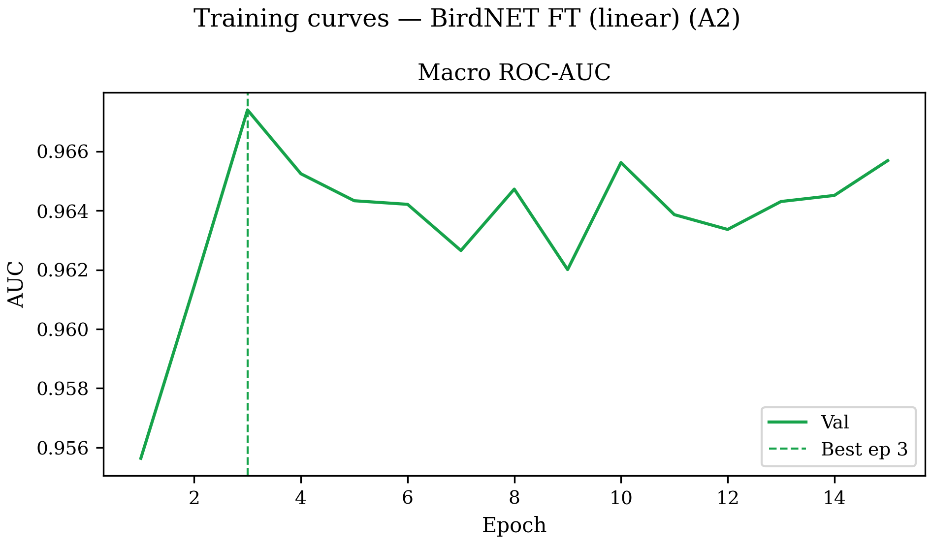
An input BatchNorm standardises the embedding scale. Both heads train for 15 epochs with AdamW (η = 10−3, weight decay 10−4), cosine annealing, a focal loss [9] (γ = 2, label smoothing ε = 0.1) with inverse-frequency class weights, a class-balanced sampler and Mixup [10]; the best validation-AUC checkpoint is restored.
REPLACE); the hidden head includes it (REPLACE_HIDDEN).Listing 6 gives the focal loss of Section 3, with label smoothing and inverse-frequency class weights.
class _FocalLoss(nn.Module):
    def __init__(self, weight=None, gamma=2.0, label_smoothing=0.1):
        super().__init__()
        self.weight, self.gamma = weight, gamma
        self.label_smoothing = label_smoothing

    def forward(self, logits, targets):
        ce = F.cross_entropy(logits, targets, weight=self.weight,
                             label_smoothing=self.label_smoothing,
                             reduction="none")
        pt = torch.exp(-ce)                          # prob of true class
        return ((1 - pt) ** self.gamma * ce).mean()
Spectrogram backbone + embedding fusion.Two ImageNet-pretrained backbones are fine-tuned and fused with the BirdNET embedding (Figure 6): an AST-style ViT-Base [5] and a ConvNeXt-Small [6]. Each maps the 224 × 224 spectrogram to a 768-d vector, concatenated with the BatchNorm-standardised 1024-d embedding and passed to a two-layer fusion head. The full stack trains for 8 epochs with AdamW (backbone lr 10−4, head lr 10−3), cosine annealing, the same focal loss and sampler, joint spectrogram/embedding mixup, and mixed precision (Listing 7).
timm returns a pooled feature vector (num_classes=0); in_chans=1 adapts the pretrained RGB stem to the mono spectrogram.class SpecEmbFusion(nn.Module):
def __init__(self, backbone_name, emb_dim, n_classes, dropout=0.3):
super().__init__()
self.backbone = timm.create_model(
backbone_name, pretrained=True, num_classes=0, in_chans=1)
self.emb_bn = nn.BatchNorm1d(emb_dim)
self.head = nn.Sequential(
nn.Linear(self.backbone.num_features + emb_dim, 512),
nn.BatchNorm1d(512), nn.GELU(), nn.Dropout(dropout),
nn.Linear(512, n_classes))
def forward(self, spec, emb):
spec = F.interpolate(spec, size=SPEC_INPUT, mode="bilinear")
feat = self.backbone(spec) # 768-d
emb = self.emb_bn(emb.float()) # 1024-d
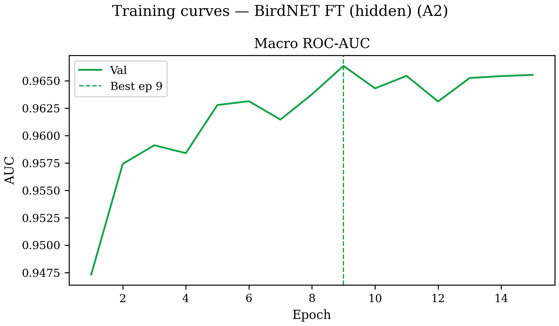
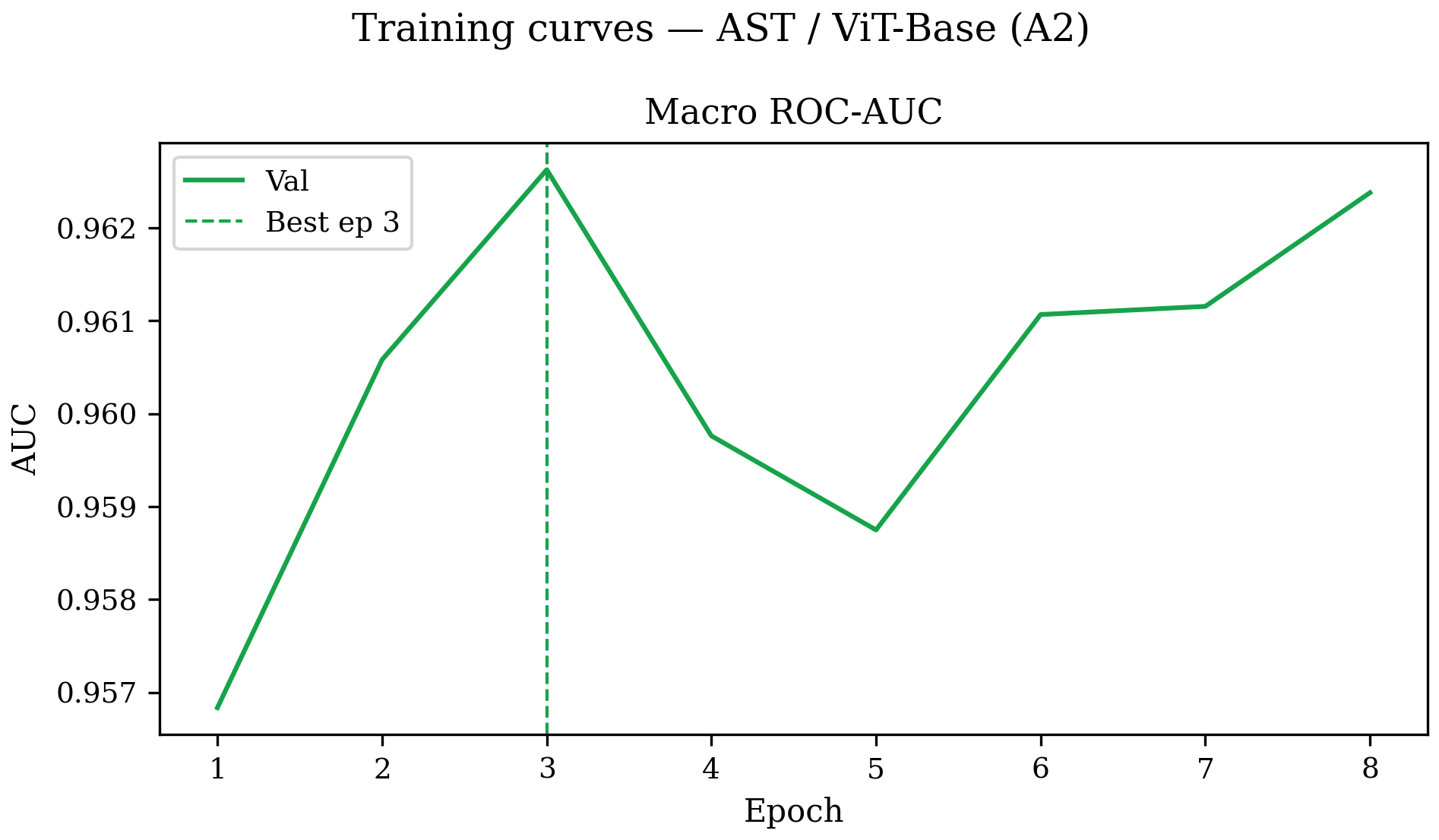
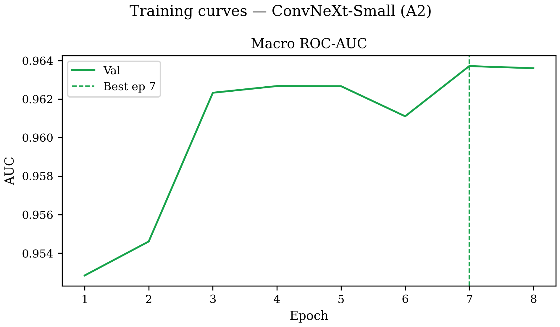
return self.head(torch.cat([feat, emb], dim=1))In the Experiment A validation curves (Figure 7), the two BirdNET heads start high and converge within a few epochs, learning only a thin classifier over BirdNET's features, while the AST/ViT and ConvNeXt backbones climb more slowly as they adapt the spectrogram mapping.
5.4From-Scratch Spectrogram CNNs
Two randomly initialized CNNs are trained on the log-mel spectrogram with no BirdNET signal (Figure 8):
- EfficientNet-B2 [7] (
tf_efficientnet_b2,in_chans=1), with a BatchNorm + Dropout(0.4) + Linear head on its 1408-d pooled features; - PANNs CNN14 [8], the standard six-block VGG-style audio CNN (channels 64→2048), each block two 3×3 conv → BN → ReLU followed by average pooling, then time-pooling, a (max + mean) frequency aggregation, a Linear(2048→2048) + ReLU, and a Dropout(0.5) + Linear output.
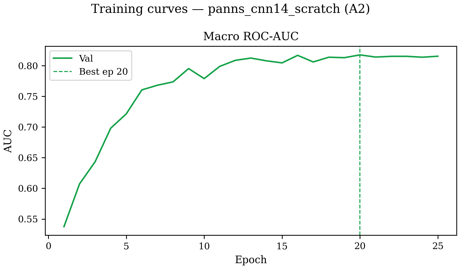
Both train for 25 epochs with Adam (η = 10−4, weight decay 10−4), cosine annealing, the same focal loss and sampler, and on-the-fly SpecAugment; the best validation checkpoint is restored. Carrying no pretrained features, they serve as a BirdNET-free baseline. Listing 8 shows the PANNs CNN14 backbone block and its (max + mean) frequency aggregation.
class _Cnn14ConvBlock(nn.Module):       # two 3x3 conv -> BN -> ReLU, then avg-pool
    def forward(self, x, pool_size=(2, 2)):
        x = F.relu_(self.bn1(self.conv1(x)))
        x = F.relu_(self.bn2(self.conv2(x)))
        return F.avg_pool2d(x, kernel_size=pool_size)

class Cnn14Bird(nn.Module):             # six blocks: 64 -> 128 -> ... -> 2048
    def features(self, x):
        x = self.bn0(x.transpose(1, 2)).transpose(1, 2)   # normalise mel bins
        for block in (self.block1, ..., self.block6):
            x = F.dropout(block(x), 0.2, self.training)
        x = torch.mean(x, dim=3)                          # pool over time
        x = torch.max(x, dim=2)[0] + torch.mean(x, dim=2) # max + mean over freq
        return F.relu_(self.fc1(F.dropout(x, 0.5, self.training)))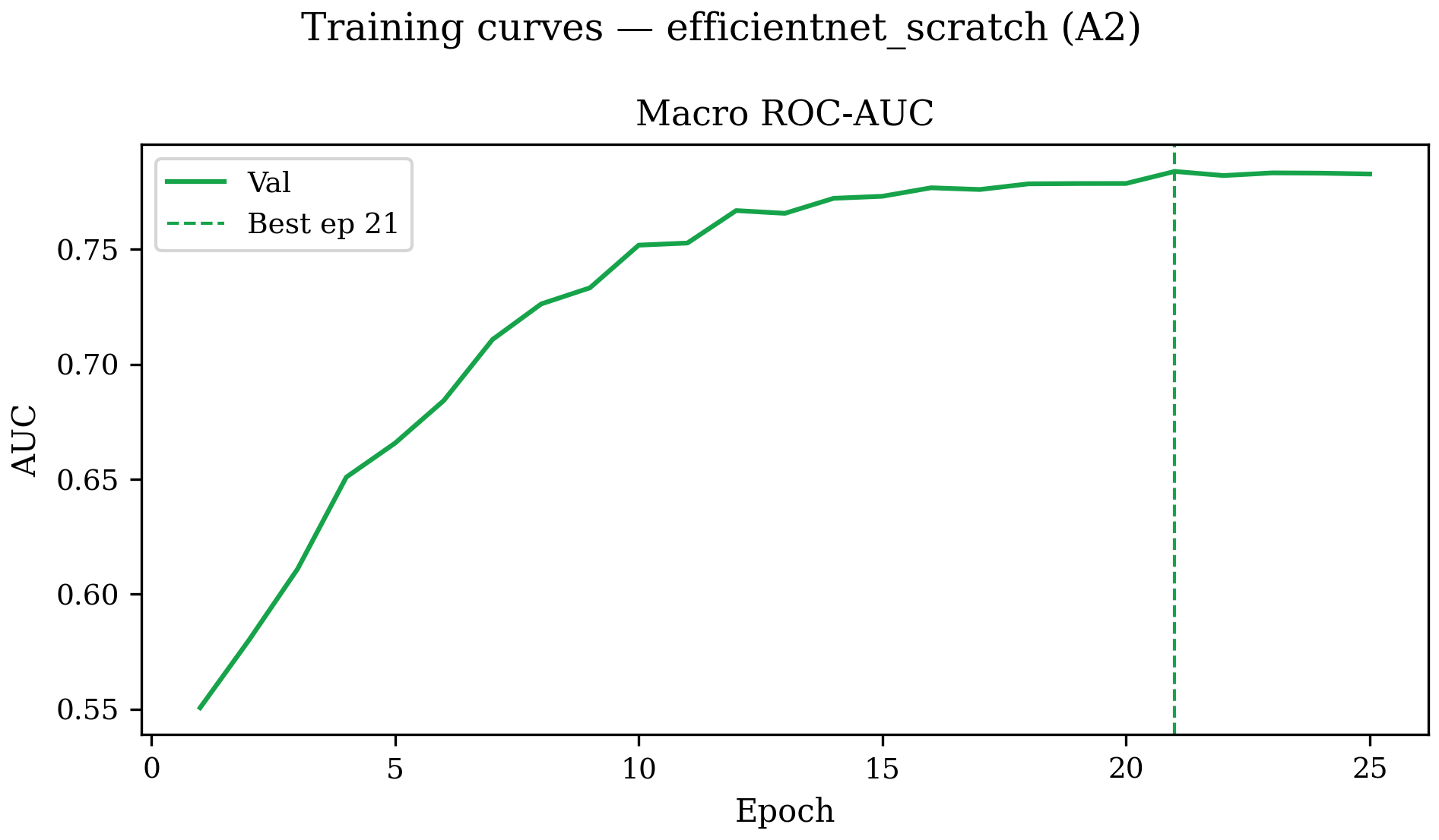
6Experiment B — AudioLDM2 Data Augmentation
6.1AudioLDM2 Synthesis Pipeline
AudioLDM2 encodes the text prompt with a CLAP encoder, runs a denoising diffusion U-Net in the latent space of a mel-spectrogram VAE, and decodes to a waveform with a HiFi-GAN vocoder (Figure 10). The pretrained pipeline runs in half precision on GPU.
Two settings control the pipeline:
- Text prompt: per species code
cls,"A field recording of a {cls} bird call in a natural environment"; - Quality filter: following the spec's verification step, a clip is kept only if the target species appears in BirdNET's top-5 predictions with confidence ≥ 0.25. Disabled by default, as it costs an extra BirdNET pass per clip for marginal gains.
6.2Synthetic Sample Generation
The per-class budget adapts to the mean intra-class embedding variance vc = 1dk=1dVari: yi=c[Xik], so acoustically diverse species receive more samples:
Listing 9 shows the generation loop: each under-represented class is topped up to its budget Tc, and every clip is resampled from AudioLDM2's native 16 kHz to the 48 kHz BirdNET expects.
var = _class_intra_variance(X_tr, y_tr_int, n_classes)
max_var = max(float(var.max()), 1.0)
for cls_str in le.classes_:
    cls_idx = int(le.transform([cls_str])[0])
    cls_target = target + int(SYNTH_EXTRA * (var[cls_idx] / max_var))
    need = max(0, cls_target - int(counts.get(cls_str, 0)))
    prompt = _species_prompt(cls_str)
    for _ in range(need):
        audio = pipe(prompt, num_inference_steps=AUDIOLDM2_STEPS,
                     audio_length_in_s=CHUNK_DUR).audios[0]
        audio = librosa.resample(audio, orig_sr=AUDIOLDM2_SR, target_sr=SR)
        sf.write(str(SYNTH_DIR / f"{cls_str}_{...}.wav"), audio, SR)
AudioLDM2 generated 3,054 synthetic samples, growing the training set from 28,436 to 31,490 examples (+10.7%), including clips for the four singleton species.
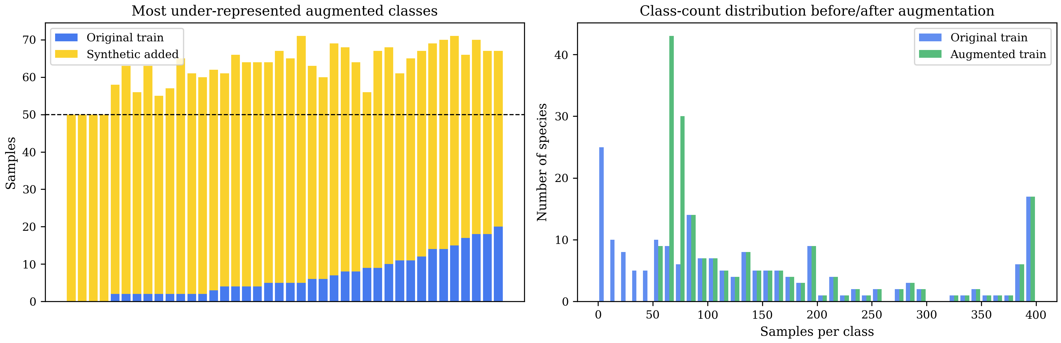
SYNTH_TARGET=50 threshold. Right: class-count histogram before and after augmentation, showing the long tail of rare species being filled in.6.3Retraining on the Augmented Data
All models of Section 5 are retrained on the augmented set with identical architecture and schedule; their validation curves follow the Experiment A pattern.
7Results
7.1Macro ROC-AUC Summary
Three patterns stand out. First, results split along the BirdNET boundary: every BirdNET-based model clears 0.96, while the from-scratch CNNs reach only 0.78–0.86, a 0.12–0.19 gap isolating the value of BirdNET's pretraining. Second, the BirdNET group is tightly clustered (0.960–0.977), so a lightweight one-hidden-layer head beats the heavier fine-tuned backbones for the best single result, 0.9770. Third, AudioLDM2 augmentation improves all nine models, modestly for the strong embedding models (+0.007 to +0.014) but largest where data is scarcest (PANNs CNN14 +0.0416).
| Model | A (original) | B (augmented) | Δ |
|---|---|---|---|
| A1/B1 — BirdNET embeddings + classical ML | |||
| LightGBM | 0.9602 | 0.9675 | +0.0073 |
| Logistic Regression | 0.9670 | 0.9757 | +0.0087 |
| MLP | 0.9614 | 0.9751 | +0.0137 |
| A2/B2 — fine-tuning | |||
| BirdNET FT (linear) | 0.9674 | 0.9763 | +0.0089 |
| BirdNET FT (hidden) | 0.9664 | 0.9770 | +0.0107 |
| AST / ViT-Base (fusion) | 0.9626 | 0.9697 | +0.0071 |
| ConvNeXt-Small (fusion) | 0.9637 | 0.9703 | +0.0066 |
| From scratch (no BirdNET) | |||
| EfficientNet-B2 | 0.7838 | 0.7934 | +0.0096 |
| PANNs CNN14 | 0.8175 | 0.8591 | +0.0416 |
7.2Per-Class Analysis
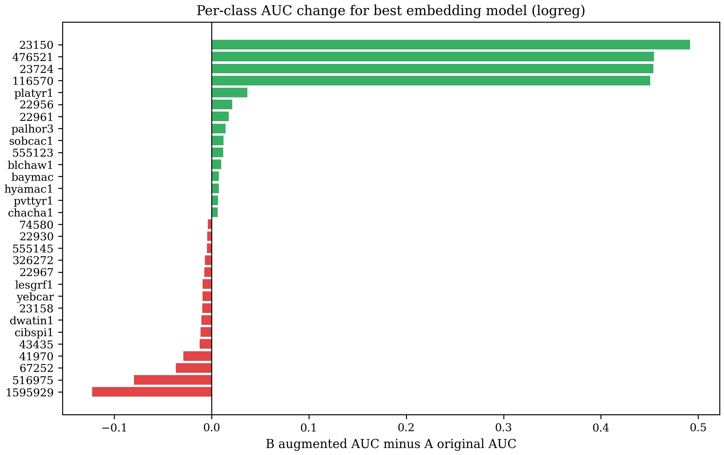
Figure 12 shows species with few original examples gain most from augmentation, while a few well-populated species degrade slightly as synthetic clips add distributional shift.
8Discussion
Choosing a from-scratch model.CNN14 out-performs EfficientNet-B2 throughout: on limited data the better from-scratch model is the better-matched audio architecture, not the larger ImageNet one.
Effect of AudioLDM2 augmentation.CNN14 gains most because, without BirdNET's features, it has the most to learn from extra data; the BirdNET models already sit near the embedding's ceiling. In well-populated classes the synthetic clips add distributional shift rather than new signal.
Singleton recovery.Synthetic clips supply the only training signal for the four validation-only singleton species, raising their predicted confidence in Experiment B.
Limitations.Four caveats temper these results. First, scores come from a single 80 / 20 split, so the sub-0.01 augmentation gains on the BirdNET heads cannot be distinguished from split noise. Second, one 3-second chunk per training file is kept for tractable runtime, discarding most of each recording. Third, AudioLDM2's text-conditioned clips are only loosely tied to true species acoustics, and the optional BirdNET top-5 verification filter (Section 6.1) is disabled by default, so part of the synthetic signal is generic “bird-like” audio. Fourth, the same split both selects each model's best checkpoint and reports its score, so the numbers are slightly optimistic.
9Conclusion
When a strong pretrained bioacoustic encoder is available, predictive performance is governed by access to its features rather than by classifier complexity: a small trained head on the frozen BirdNET embedding achieves the best result (0.9770 macro-AUC), matching or beating heavyweight fusion backbones and exceeding the from-scratch CNNs by 0.12–0.19. AudioLDM2 augmentation is a reliable, architecture-agnostic add-on: it improves every model tested, helps most where data is scarcest, and uniquely supplies training signal for the otherwise-unseen singleton classes.
References
- [1]Cornell Lab of Ornithology. BirdCLEF 2026. Kaggle competition, 2026.
https://www.kaggle.com/competitions/birdclef-2026. - [2]Haohe Liu, Yi Yuan, Xubo Liu, Xinhao Mei, Qiuqiang Kong, Qiao Tian, Yuping Wang, Wenwu Wang, Yuxuan Wang, and Mark D Plumbley. Audioldm 2: Learning holistic audio generation with self-supervised pretraining. IEEE/ACM Transactions on Audio, Speech, and Language Processing, 32:2871–2883, 2024.
- [3]Stefan Kahl, Connor M Wood, Maximilian Eibl, and Holger Klinck. Birdnet: A deep learning solution for avian diversity monitoring. Ecological Informatics, 61:101236, 2021.
- [4]Stefan Kahl, Amanda Navine, Tom Denton, Holger Klinck, Patrick Hart, Hervé Glotin, Hervé Goëau, Willem-Pier Vellinga, Robert Planqué, and Alexis Joly. Overview of birdclef 2022: Endangered bird species recognition in soundscape recordings. CEUR-WS, 2022.
- [5]Yuan Gong, Yu-An Chung, and James Glass. Ast: Audio spectrogram transformer. arXiv preprint arXiv:2104.01778, 2021.
- [6]Zhuang Liu, Hanzi Mao, Chao-Yuan Wu, Christoph Feichtenhofer, Trevor Darrell, and Saining Xie. A convnet for the 2020s. In Proceedings of the IEEE/CVF conference on computer vision and pattern recognition, pages 11976–11986, 2022.
- [7]Mingxing Tan and Quoc Le. Efficientnet: Rethinking model scaling for convolutional neural networks. In International conference on machine learning, pages 6105–6114. PMLR, 2019.
- [8]Qiuqiang Kong, Yin Cao, Turab Iqbal, Yuxuan Wang, Wenwu Wang, and Mark D Plumbley. Panns: Large-scale pretrained audio neural networks for audio pattern recognition. IEEE/ACM Transactions on Audio, Speech, and Language Processing, 28:2880–2894, 2020.
- [9]Tsung-Yi Lin, Priya Goyal, Ross Girshick, Kaiming He, and Piotr Dollár. Focal loss for dense object detection. In Proceedings of the IEEE international conference on computer vision, pages 2980–2988, 2017.
- [10]Hongyi Zhang, Moustapha Cisse, Yann N Dauphin, and David Lopez-Paz. mixup: Beyond empirical risk minimization. arXiv preprint arXiv:1710.09412, 2017.
- [11]Daniel S Park, William Chan, Yu Zhang, Chung-Cheng Chiu, Barret Zoph, Ekin D Cubuk, and Quoc V Le. Specaugment: A simple data augmentation method for automatic speech recognition. arXiv preprint arXiv:1904.08779, 2019.
- [12]Guolin Ke, Qi Meng, Thomas Finley, Taifeng Wang, Wei Chen, Weidong Ma, Qiwei Ye, and Tie-Yan Liu. Lightgbm: A highly efficient gradient boosting decision tree. Advances in neural information processing systems, 30, 2017.