Queueing for engineers: Little’s law, utilisation and tail latency

A service that is comfortable at 70% CPU can be unusable at 90%, even though it is nowhere near full. Nothing broke; the latency came from queueing, and queueing grows non-linearly with load. A few results from queueing theory explain most capacity surprises: why latency rises the way it does, why some systems tolerate high utilisation and others don’t, and how big a pool should be.

This article covers Little’s law, how waiting time depends on utilisation and variability, why a shared queue beats many separate ones, what queues do to tail latency, how to size connection and thread pools, and what to do when arrivals exceed capacity. The maths is light, and every result here is something you can check against your own dashboards.

Little’s law

For any stable system, the average number of things in it equals the rate they arrive multiplied by the average time each one spends inside:

It holds whatever the distribution of arrivals or service times, for any boundary you draw: a single queue, a server, a whole service. That makes it a conversion tool between the three numbers you can usually measure.

• A service handling 2,000 requests per second with a mean latency of 50 ms has, on average, 100 requests in flight. If its thread pool has 64 threads, something has to be queueing.
• A database pool that serves 800 queries per second, each holding a connection for 20 ms, keeps 16 connections busy on average. That is the floor for the pool size, not the answer.
• A Kafka consumer group with a lag of 60,000 messages, consuming 1,000 per second, is about a minute behind.

Little’s law says nothing about variance, though: it gives averages. To know how much queueing happens, you need a model of how arrivals and work vary.

Utilisation and the hockey stick

The simplest useful model is the M/M/1 queue: one server, requests arriving at random (a Poisson process), and service times drawn from an exponential distribution with mean S. With utilisation ρ, the fraction of time the server is busy, the mean time in the system is:

At 50% utilisation a request takes on average twice its service time. At 80%, five times. At 90%, ten; at 95%, twenty; at 99%, a hundred. Each halving of the idle capacity doubles the latency.

The intuition: requests don’t arrive evenly. At any utilisation below 100% there are idle gaps, and random clumps of arrivals form queues that the server only works off during those gaps. As utilisation rises, the gaps shrink, so each clump takes longer to clear, and the next clump often arrives before it has.

Variability is the multiplier

Real systems aren’t M/M/1, but Kingman’s formula approximates the mean queueing delay of a single server with any arrival and service distributions:

The first factor is the utilisation term from before. The second is variability: c_a and c_s are the coefficients of variation (standard deviation over mean) of the gaps between arrivals and of the service times. Random arrivals and exponential service give 1 for each; perfectly regular service gives c_s = 0 and halves the wait.

This is the more practical result. A service whose requests are all roughly the same cost can run hotter than one where 1% of requests are a hundred times more expensive, because those expensive requests make c_s large and every cheap request behind them waits. Bursty arrivals, from batch jobs, cron schedules, retries or synchronised clients, raise c_a in the same way. Two ways to buy back latency without adding capacity follow directly: separate the expensive work into its own queue, and smooth the bursts.

Where work waits

Give the same four servers the same load, and the waiting time still depends heavily on how work reaches them:

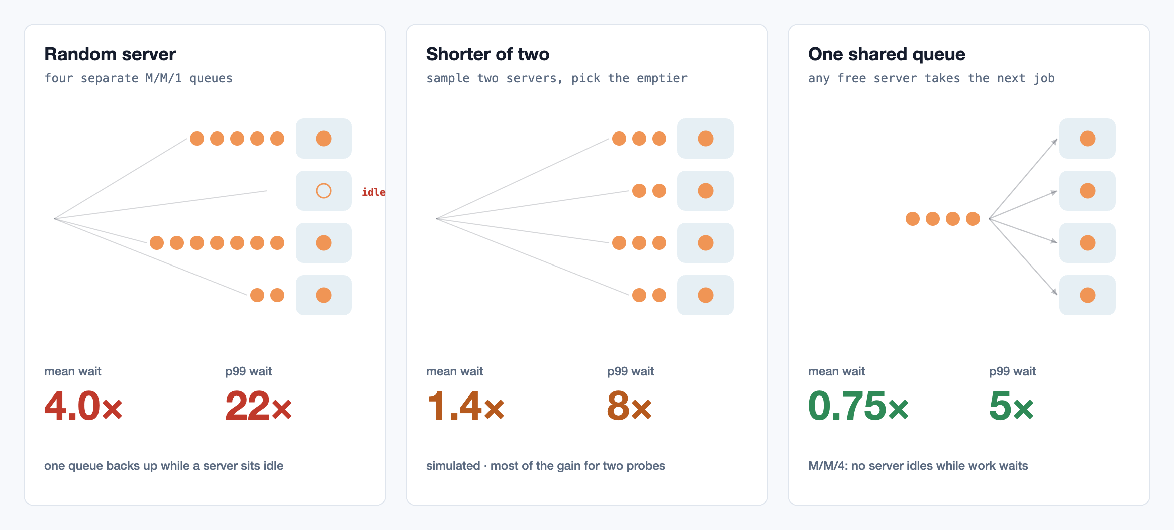
• Separate queues with random assignment behave like four independent M/M/1 queues, each at 80%. Luck decides which queue a request joins.
• One shared queue (the M/M/c model) waits five times less on average, because no server is ever idle while a request is waiting. This is why a single run queue feeding a thread pool beats per-thread queues, and why one large pool usually beats several small ones at the same total size.
• The power of two choices: when a shared queue isn’t possible, as with a load balancer in front of many servers, sampling two servers at random and sending the request to the less loaded one recovers most of the difference. Least-outstanding-requests balancing works for the same reason.

Queues and tail latency

Queueing hurts percentiles more than averages. In an M/M/1 queue the response time is exponentially distributed, so the 99th percentile is ln(100) ≈ 4.6 times the mean. At 90% utilisation that is 46 times the service time; a 10 ms operation has a p99 near half a second, with nothing wrong except load.

Two consequences show up in distributed systems. First, a service whose latency SLO is on p99 must run at lower utilisation than one that only cares about the mean. Second, a request that fans out to many backends waits for the slowest, so it feels the backends’ tails rather than their averages; the arithmetic of that is in the article on microservices.

Sizing connection and thread pools

A connection pool is a queue in front of a fixed number of servers: requests wait for a connection, then hold it while their query runs. Little’s law gives the minimum: arrival rate × time each connection is held. Queueing theory gives the margin above it needed to keep the wait for a connection small, which the calculator below computes.

The counterintuitive part is the upper bound. The connections are not the real servers; the database’s CPU cores and disks are. A database with 16 cores can only run 16 queries at once. With 200 connections all active, the extra queries don’t run faster; they compete for the same cores, add context switching and lock contention, and make every query slower. Raising the pool size during an incident usually makes it worse. A useful starting point, from the HikariCP project’s guidance, is about twice the database’s core count, then measure.

The same reasoning sets thread pools, worker counts and concurrency limits. A limit equal to the downstream system’s real parallelism, with a short, bounded queue in front, gives better latency than a large limit that lets work pile up inside the downstream instead.

When arrivals exceed capacity

The formulas above assume ρ < 1. When work arrives faster than it can be served, there is no steady state: the queue grows without bound, and so does latency. Every request eventually waits longer than its client is willing to, so the server spends all its capacity on work nobody is waiting for any more. Throughput of useful work, goodput, collapses even though the server is 100% busy.

The defences all come down to one idea: limit how much waiting the system is willing to do. Keep queues bounded and reject early, since a fast “no” can be retried elsewhere while a slow failure just burns capacity; drop work whose deadline has already passed; and don’t let retries add load at the moment the system is full. Those techniques, from load shedding and CoDel-style queues to retry budgets and circuit breakers, are covered in the article on retries and circuit breakers, and keeping one client from using all the headroom in the article on rate limiting.

Planning headroom

So how hot should a service run? It depends on three things the models make explicit: the latency objective and which percentile it is on, how variable the workload is, and how many servers share the load. A large pool of identical workers serving uniform requests can run at 80% or more; a single-threaded component with occasional very expensive requests may need to stay under 50% to meet a p99 target.

Two more allowances sit on top. Capacity must survive losing a zone or region, so a service that runs at 60% across three zones is at 90% when one fails (see the article on multi-region). And utilisation is usually measured as an average over a minute, which hides the short bursts where queues form. The per-second peak is what the queue sees.

The practical method: run a load test that steps the arrival rate up, plot p50 and p99 latency against throughput, and find the knee. Then operate well to the left of it, alert on queueing delay directly, and scale on it rather than on CPU alone.

A capacity calculator

Erlang C gives the probability of waiting in an M/M/c queue; from it come the mean and p99 queueing delay, Little’s law gives the number in flight, and a short search finds the smallest pool that keeps the p99 wait within a budget. For 800 queries per second holding a connection for 20 ms, 17 connections give a p99 wait of about 86 ms, 20 give 16 ms, and 24 bring it under 4 ms.

// M/M/c: Poisson arrivals, exponential service times, c servers sharing one FIFO queue.
// Rough for real systems, but it gives the right shape and the right order of magnitude.

/** Probability that an arrival has to wait (Erlang C). a = λ/μ, the load in servers' worth of work. */
export function erlangC(c: number, a: number): number {
  if (a >= c) return 1;
  let term = 1;
  let sum = 1;
  for (let k = 1; k < c; k++) {
    term *= a / k; // a^k / k!
    sum += term;
  }
  const last = (term * a) / c / (1 - a / c); // a^c / c! · 1/(1-ρ)
  return last / (sum + last);
}

type Estimate = { utilisation: number; meanWaitMs: number; p99WaitMs: number; inFlight: number };

/** Queueing delay for c workers, each taking serviceMs per job on average, at rate arrivals per second. */
export function estimate(c: number, rate: number, serviceMs: number): Estimate {
  const mu = 1000 / serviceMs; // jobs per second per worker
  const a = rate / mu;
  const rho = a / c;
  if (rho >= 1) return { utilisation: rho, meanWaitMs: Infinity, p99WaitMs: Infinity, inFlight: Infinity };
  const pWait = erlangC(c, a);
  const drain = c * mu - rate; // the rate at which a backlog clears
  const meanWaitMs = (1000 * pWait) / drain;
  // P(wait > t) = pWait · e^(-drain·t), so the 99th percentile wait is:
  const p99WaitMs = pWait <= 0.01 ? 0 : (1000 * Math.log(pWait / 0.01)) / drain;
  // Little's law: jobs in the system = arrival rate × time in the system.
  const inFlight = rate * ((meanWaitMs + serviceMs) / 1000);
  return { utilisation: rho, meanWaitMs, p99WaitMs, inFlight };
}

/** The smallest pool that keeps p99 queueing delay under a budget at the given rate. */
export function poolSize(rate: number, serviceMs: number, p99BudgetMs: number): number {
  let c = Math.max(1, Math.ceil((rate * serviceMs) / 1000)); // fewer than this can't keep up at all
  while (estimate(c, rate, serviceMs).p99WaitMs > p99BudgetMs) c++;
  return c;
}

// 800 queries/s holding a connection for 20 ms each: 16 connections' worth of work.
for (const c of [17, 18, 20, 24, 32]) console.log(c, estimate(c, 800, 20));
console.log("pool for p99 wait under 5 ms:", poolSize(800, 20, 5));

References

1. Little, J. D. C. (1961). A Proof for the Queuing Formula: L = λW. Operations Research. doi:10.1287/opre.9.3.383
2. Kingman, J. F. C. (1961). The single server queue in heavy traffic. Mathematical Proceedings of the Cambridge Philosophical Society. doi:10.1017/S0305004100036094
3. Harchol-Balter, M. (2013). Performance Modeling and Design of Computer Systems: Queueing Theory in Action. Cambridge University Press. cs.cmu.edu/~harchol
4. Mitzenmacher, M. (2001). The Power of Two Choices in Randomized Load Balancing. IEEE Transactions on Parallel and Distributed Systems. doi:10.1109/71.963420
5. Dean, J. & Barroso, L. A. (2013). The Tail at Scale. Communications of the ACM. doi:10.1145/2408776.2408794
6. Nichols, K. & Jacobson, V. (2012). Controlling Queue Delay. ACM Queue. queue.acm.org
7. Brett Wooldridge. About Pool Sizing. HikariCP wiki. github.com/brettwooldridge/HikariCP/wiki/About-Pool-Sizing